If you've never used a spreadsheet to create documents before, we recommend reading our guide to Excel for Dummies.
You'll then be able to create your first spreadsheet with tables, graphs, math formulas, and formatting.
Details about basic functions and the capabilities of the MS Excel spreadsheet processor. Description of the main elements of the document and instructions for working with them in our material.

Working with cells. Filling and formatting
Before proceeding with specific actions, you need to understand the basic element of any document in Excel. An Excel file consists of one or several sheets divided into small cells.
A cell is a basic component of any Excel report, table or graph. Each cell contains one block of information. This could be a number, date, monetary amount, unit of measurement, or other data format.
To fill a cell, just click on it with the pointer and enter necessary information. To edit a previously filled cell, double-click on it.
Rice. 1 – example of filling cells
Each cell on the sheet has its own unique address. Thus, you can carry out calculations or other operations with it. When you click on a cell, a field will appear at the top of the window with its address, name and formula (if the cell is involved in any calculations).
Select the “Share of Shares” cell. Its location address is A3. This information is indicated in the properties panel that opens. We can also see the content. This cell has no formulas, so they are not shown.
More cell properties and functions that can be applied to it are available in context menu. Click on the cell with the right mouse button. A menu will open with which you can format the cell, analyze the contents, assign a different value, and other actions.
Rice. 2 – context menu of the cell and its main properties
Sorting data
Often users are faced with the task of sorting data on a sheet in Excel. This feature helps you quickly select and view only the data you need from the entire table.
In front of you is an already filled out table (we’ll figure out how to create it later in the article). Imagine that you need to sort data for January in ascending order. How would you do it? Simply retyping a table is extra work, and if it is large, no one will do it.
There is a special function for sorting in Excel. The user is only required to:
- Select a table or block of information;
- Open the “Data” tab;
- Click on the “Sorting” icon;
Rice. 3 – “Data” tab
- In the window that opens, select the table column on which we will perform actions (January).
- Next is the sorting type (we group by value) and, finally, the order - ascending.
- Confirm the action by clicking on “OK”.
Rice. 4 – setting sorting parameters
The data will be sorted automatically:
Rice. 5 – the result of sorting the numbers in the “January” column
Similarly, you can sort by color, font and other parameters.
Mathematical calculations
The main advantage of Excel is the ability to automatically carry out calculations while filling out the table. For example, we have two cells with values 2 and 17. How can we enter their result into the third cell without doing the calculations ourselves?
To do this, you need to click on the third cell in which the final result of the calculations will be entered. Then click on the function icon f(x) as shown in the image below. In the window that opens, select the action you want to apply. SUM is the sum, AVERAGE is the average, and so on. Full list functions and their names in the Excel editor can be found on the official website Microsoft.
We need to find the sum of two cells, so click on “SUM”.
Rice. 6 – select the “SUM” function
There are two fields in the function arguments window: “Number 1” and “Number 2”. Select the first field and click on the cell with the number “2”. Its address will be written into the argument line. Click on “Number 2” and click on the cell with the number “17”. Then confirm the action and close the window. If you need to perform mathematical operations on three or more cells, simply continue entering the argument values in the Number 3, Number 4, and so on fields.
If in further meaning The summed cells will change, their sum will be updated automatically.
Rice. 7 – result of calculations
Creating tables
You can store any data in Excel tables. Using the function quick setup and formatting, it is very easy to organize a control system in the editor personal budget, list of expenses, digital data for reporting, etc.
Tables in Excel have an advantage over a similar option in Word and others office programs. Here you have the opportunity to create a table of any size. The data is easy to fill out. There is a function panel for editing content. In addition, the finished table can be integrated into a docx file using the usual copy-paste function.
To create a table, follow the instructions:
- Open the Insert tab. On the left side of the options panel, select Table. If you need to consolidate any data, select the “Pivot Table” item;
- Using the mouse, select the space on the sheet that will be allocated for the table. And also you can enter the location of the data in the element creation window;
- Click OK to confirm the action.
Rice. 8 – creating a standard table
To format appearance the resulting sign, open the contents of the designer and in the “Style” field, click on the template you like. If desired, you can create your own view with a different color scheme and cell highlighting.
Rice. 9 – table formatting
Result of filling the table with data:
Rice. 10 – completed table
For each table cell, you can also configure the data type, formatting, and information display mode. The designer window contains all the necessary options for further configuration of the sign, based on your requirements.
Adding graphs/charts
To build a chart or graph, you need to have a ready-made plate, because graphical data will be based precisely on information taken from individual rows or cells.
To create a chart/graph you need:
- Select the table completely. If a graphic element needs to be created only to display the data of certain cells, select only them;
- Open the insert tab;
- In the recommended charts field, select the icon that you think will best visually describe the tabular information. In our case, this is a three-dimensional pie chart. Move the pointer to the icon and select the appearance of the element;
In a similar way, you can create scatter plots, line diagrams, and table element dependency diagrams. All received graphic elements can also be added to text documents Word.
The Excel spreadsheet editor has many other functions, however, the techniques described in this article will be sufficient for initial work. In the process of creating a document, many users independently master more advanced options. This happens thanks to a convenient and intuitive interface latest versions programs.
Thematic videos:
Microsoft Excel- one of the most popular spreadsheet editors, allowing you to do any mathematical calculations and use complex formulas to calculate the required quantities. The Excel editor has a huge library of formulas for various types of tasks: continuing a number series, finding the average value from a number of available ones, drawing up proportions, solving and analyzing linear and nonlinear equations and other functions for the corresponding purpose.
Capabilities of the Microsoft Excel spreadsheet processor
In one of their key projects, the developers introduced the following set of abilities:
- an expanded arsenal of formatting cell contents in Excel. You can choose the color and typeface of the font, text style, border, fill color, alignment; decreasing and increasing indentation. Finally, the utility allows you to set the number format of cells with a decrease or increase in bit depth; inserting, deleting and moving cells; calculation of the aggregated amount; sorting and filtering by specified criteria and other options
- insert a huge number of charts and graphs to analyze and visualize numerical data. Thus, the standard functionality of Excel allows you to insert illustrations, pivot tables, histograms or bar charts into a sheet; hierarchical, waterfall and radar charts. In addition to this, the use of area graphs is available; statistical, combination and donut charts, as well as a special subtype of dot or bubble sparklines
- a page layout tool similar to Word. The user is able to configure margins, orientation and page size; select an individual theme from the built-in library or downloaded from the network; customize the colors, fonts, and effects that apply to table content; width, height and scale of printouts and other elements
- wide range of products presented in the program Excel functions. All functions are divided into appropriate categories, making them easy to use and select. You can also create formula dependencies that clearly demonstrate which cells affect the calculation of the resulting values in the desired slot
- obtaining external data from third-party sources for use in relational databases. A nested Excel function set allows you to immediately generate a query for transfer to a DBMS from an external file, web services, ODBC container and other sources
- built-in advanced review and collaboration tools. Readers and editors can simultaneously open the same document once it's synced to the cloud, make changes and edits, and add comments for other reviewers
- integrated engine for checking spelling, thesaurus, syntax and punctuation of the typed text. If a given module encounters a new term or phrase, it is immediately underlined so that the author of the document is aware of the possible error.
On this portal, you can select any version of the Excel editor to download by going to the page of the current edition of the program and clicking on the active link. All software on the site is available absolutely free and contains Russian localization.
If for the constructed chart there is new data on the sheet that needs to be added, then you can simply select the range with the new information, copy it (Ctrl + C) and then paste it directly into the chart (Ctrl + V).
Suppose you have a list of full names (Ivanov Ivan Ivanovich), which you need to turn into abbreviated ones (Ivanov I. I.). To do this, you just need to start writing the desired text in the adjacent column manually. On the second or third Excel line will try to predict our actions and perform further processing automatically. All you have to do is press the Enter key to confirm, and all names will be converted instantly. In a similar way, you can extract names from email, merge full names from fragments, and so on.

You most likely know about the magic autofill marker. This is a thin black cross in the lower right corner of a cell, by pulling it you can copy the contents of the cell or a formula to several cells at once. However, there is one unpleasant nuance: such copying often violates the design of the table, since not only the formula is copied, but also the cell format. This can be avoided. Immediately after pulling the black cross, click on the smart tag - a special icon that appears in the lower right corner of the copied area.
If you select the “Copy values only” option (Fill Without Formatting), Excel will copy your formula without formatting and will not spoil the design.

In Excel, you can quickly display your geodata, such as sales by city, on an interactive map. To do this, you need to go to the “App Store” (Office Store) on the “Insert” tab and install the “Bing Maps” plugin from there. This can also be done from the site by clicking the Get It Now button.
After adding a module, you can select it from the My Apps drop-down list on the Insert tab and place it on your worksheet. All you have to do is select your data cells and click on the Show Locations button in the map module to see our data on it. If desired, in the plugin settings you can select the type of chart and colors to display.

If the number of worksheets in a file exceeds 10, then it becomes difficult to navigate through them. Right-click on any of the sheet tab scroll buttons in the lower left corner of the screen. A table of contents will appear, and you can go to any desired sheet instantly.

If you've ever had to manually move cells from rows to columns, you'll appreciate the following trick:
- Select a range.
- Copy it (Ctrl + C) or by right-clicking and select “Copy”.
- Right-click the cell where you want to paste the data and select one of the paste special options from the context menu - the Transpose icon. Older versions of Excel do not have this icon, but you can solve the problem by using Paste Special (Ctrl + Alt + V) and selecting the Transpose option.

If in any cell you are supposed to enter strictly defined values from the allowed set (for example, only “yes” and “no” or only from a list of company departments, and so on), then this can be easily organized using a drop-down list.

- Select the cell (or range of cells) that should contain such a restriction.
- Click the “Data Validation” button on the “Data” tab (Data → Validation).
- In the “Type” drop-down list, select the “List” option.
- In the “Source” field, specify a range containing reference variants of elements that will subsequently appear as you enter.

If you select a range with data and on the “Home” tab click “Format as Table” (Home → Format as Table), then our list will be converted into a smart table that can do a lot of useful things:
- Automatically expands when new rows or columns are added to it.
- The entered formulas will be automatically copied to the entire column.
- The header of such a table is automatically fixed when scrolling, and it includes filter buttons for selection and sorting.
- On the “Design” tab that appears, you can add a total line with automatic calculation to such a table.

Sparklines are miniature diagrams drawn directly in cells that visually display the dynamics of our data. To create them, click the Line or Columns button in the Sparklines group on the Insert tab. In the window that opens, specify the range with the original numerical data and the cells where you want to display sparklines.

After clicking the “OK” button, Microsoft Excel will create them in the specified cells. On the “Design” tab that appears, you can further configure their color, type, enable the display of minimum and maximum values, and so on.
Imagine: you close the report you've been fiddling with for the last half of the day, and the "Save changes to file?" dialog box appears. suddenly for some reason you press “No”. The office is filled with your heart-rending scream, but it’s too late: the last few hours of work have gone down the drain.
In fact, there is a chance to improve the situation. If you have Excel 2010, then click on “File” → “Recent” (File → Recent) and find the “Recover Unsaved Workbooks” button in the lower right corner of the screen.
In Excel 2013, the path is slightly different: “File” → “Information” → “Version Control” → “Recover Unsaved Workbooks” (File - Properties - Recover Unsaved Workbooks).
In later versions of Excel, open File → Details → Manage Workbook.

A special folder from the depths will open Microsoft Office, where, in such a case, temporary copies of all created or modified but unsaved books are saved.
Sometimes when working in Excel, you need to compare two lists and quickly find the elements that are the same or different. Here is the fastest and most visual way to do this:
- Select both columns to compare (hold down the Ctrl key).
- Select on the Home tab → Conditional Formatting → Highlight Cell Rules → Duplicate Values.
- Select the Unique option from the drop-down list.

Have you ever tweaked the input values in your Excel calculation to get the output you want? At such moments, you feel like a seasoned artilleryman: just a couple of dozen iterations of “undershooting - overshooting” - and here it is, the long-awaited hit!
Microsoft Excel can do this adjustment for you, faster and more accurately. To do this, click the “What If Analysis” button on the “Data” tab and select the “Parameter Selection” command (Insert → What If Analysis → Goal Seek). In the window that appears, specify the cell where you want to select the desired value, the desired result and the input cell that should change. After clicking “OK,” Excel will perform up to 100 “shots” to find the total you require with an accuracy of 0.001.

Description Reviews (0) Screenshots
- availability of functions for quickly obtaining access to the requested data with the ability to store them in a specific location;
- ability to make forecasts using the exponential smoothing method;
- presence of basic forecasting parameters in the settings;
- the ability to geoposition with launch from the workspace, as well as free download of the XL program;
- cost tracking with a detailed report on income and expenses using the added “analysis” and “balance” templates;
- analysis of changes in stock performance that occurred over an arbitrarily selected period of time;
- Availability of Power BI, which allows publishing the project;
- instant formatting of a table with a diagram thanks to the function quick change figure parameters.
Microsoft Excel 2016 is popular program, allowing edit spreadsheets, significantly improved and received a number of additional functionality, which can only be fully used by subscribers . IN new version 2016 applications, if you download the XL program, there are diagrams that help efficient work with any projects, using the demonstration of statistical data and their hierarchy.

Advantages and Features of Excel
The advantages of the free downloaded XLS program should be noted:
When you download the XLSX program for free, the new version will contain the “What do you want to do?” field, the use of which in your work significantly reduces the time it takes to complete the task. Here you need to designate a command or function, after which the editor will select a specific menu necessary for further work. Another innovation is handwriting input with the touch of a finger or stylus for devices with touch screens. If such a device is not available, you can use a mouse.
Functional
A convenient, although unusual at first glance, menu provides maximum comfort when working with tables. Besides, in Excel versions 2007, taking into account the wishes of users of versions 1997-2003, were increased permissible dimensions tables due to additional rows and columns.
With the release of Excel 2007, all imperfections were eliminated thanks to a radically new approach to the issue of interface development. And although this version has been available to users for more than six years; it has not lost its position in the software market to this day. An all-new, user-centric interface in Excel 2007 not available in previous versions, brought this Microsoft product to a leading position.