The formula bar is a special line located above the column headings and intended for entering and editing formulas and other information. A fragment of the formula bar is shown in Figure 3.4.
Figure 3.4 - Formula bar
The formula bar consists of two main parts: the address bar, which is located on the left, and the line for entering and displaying information. In Figure 3.4, the name of the last used function (in this case, the sum calculation function) is displayed in the address bar, and the formula “=A1+5” is displayed in the information entry and display line.
The address line is designed to display the address of the selected cell or range of cells, as well as to enter the required addresses from the keyboard. However, when you select a group of cells, the address bar will only show the address of the first cell in the range, located in its upper left corner.
In the Excel 2007 spreadsheet editor, you can fully automate calculations using the “Formula” data type. Formula is a special tool of Excel 2007 designed for calculations, calculations and data analysis.
The formula begins with the "=" sign, followed by operands and operators. List arithmetic operators is given in table 3.1. The precedence of operations when calculating Excel formulas is as follows:
− telecom operators (performed first);
− operator percentage;
− unary minus;
− exponentiation operator;
− multiplication and division operators;
− addition and subtraction operators (last). Table 3.1 - Symbols for indicating operators in Excel

take a percentage |
||
exponentiation |
||
Telecom operators |
||
range setting |
SUM(A1:B10) |
|
Union |
SUM(A1;A3) |
Brackets in Excel formulas perform the usual, from an algebraic point of view, role of indicating the priority of calculating a particular part of the expression. For example:
= 10*4+4^2 gives the result 56
= 10*(4+4^2) gives the result 200
Particular care must be taken when placing parentheses when specifying a unary minus. For example: = -10^2 gives the result 100, and =-(10^2) gives the result -100; - 1^2+1^2 gives the result 2, and 1^2-1^2 gives the result 0.
If the formula cannot be calculated correctly, Excel displays an error code in the cell instead of the expected result (Table 3.2).
Table 3.2 – Error messages when calculating formulas
Error code |
|
The formula attempts to divide by zero (empty cells |
|
are considered zeros) |
|
No value available |
|
The name used in the formula is not recognized |
|
but the intersection of two areas that do not have common cells) |
|
A function with a numeric argument uses inappropriate |
|
argument |
|
Formula incorrectly references cell |
|
Invalid argument type used |
Functions in Excel
You can also perform many types of calculations using special built-in functions in Excel 2007. A function is a procedure originally created and embedded in the Excel program that performs calculations based on given arguments in a certain order.
Each function must include the following elements: name or title (examples of names - SUM, AVERAGE, COUNT, MAX, etc.), as well as an argument (or several arguments), which is specified in parentheses immediately after the function name . Function arguments can be numbers, links, formulas, text, logical values etc.. If the argument is
The function has several components, they are specified separated by commas. If a function has no arguments, for example, the PI() function, then nothing is specified inside the brackets. Parentheses allow you to define where the argument list begins and ends. You cannot insert anything between the function name and the parentheses. Therefore, the symbol for raising a function to a power is given after writing the argument. For example, SIN(A1)^3. If the rules for writing a function are violated, Excel displays a message stating that there is an error in the formula.
You can enter functions either manually or automatic mode. In the latter case, use the function wizard, which opens with the button Insert function, which is located on the Excel 2007 ribbon on the Formulas tab.
All functions available in the program are grouped into categories for ease of use. The category is selected from the Category drop-down list, and a list of functions included in this category is displayed at the bottom of the window. If you select the required function and press the OK button, a window will open (its contents depend on the specific function) in which the function arguments are indicated.
IN engineering calculations Trigonometric functions are often used. Please note that the argument of the trigonometric function must be specified in radians. Therefore, if the argument is given in degrees, it must be converted to radians. This can be implemented either through the conversion formula “=A1*PI()/180” (assuming that the argument is written in the cell with address A1), or using the RADIANS(A1) function.
Example. Write the Excel formula = − for2 + calculation3 1+e function tg 3 (5 2 ) b .
Assuming that x is in degrees and is in cell A1 and b is in cell B1, the formula in Excel cell will look like this:
=(- (B1^2) + (1+exp(B1))^(1/3)) /TAN(5*RADIANS(A1)^2) ^3
Relative and absolute cell addresses
To register in Excel formulas absolute cell addressing should be used for constants. In this case, when copying the formula to another cell, the address of the cell with the constant will not change. To change the relative address of cell B2 to the absolute $B$2 in the formula, you must successively press the F4 key, or manually add dollar symbols. There are also mixed cell addresses (B$2 and $B2). When copying a formula containing

mixed addresses, only the part of the address that is not fixed (with the $ sign on the left) is changed.
When you copy a formula into an adjacent cell along a row, the letter component changes in the relative link address. For example, link A3 will be replaced by link B3, but the mixed address $A1 will not change when copied along the line. Accordingly, when copying a formula into an adjacent cell in a column in the relative link address, the digital component changes. For example, link A1 will be replaced by link A2, but the mixed address A$1 will not change when copied along the column.
Building charts
In Excel, the term chart refers to any graphical representation numerical data. Charts are built based on a data series - a group of cells with data within one row or column. You can display multiple data series on one chart.
The easiest way to create charts is as follows: select one or more data series, and in the Charts group of the Insert tab of the Excel ribbon, select the desired chart type. The diagram will be placed on the current sheet of the workbook. If necessary, it can be transferred to another sheet using the command Move chart tabs Designer for working with diagrams. Using the tab Layout Working with diagrams
you can change the appearance of the chart: add the title of the chart, axes, change fonts, etc. If necessary, you can change the captions to horizontal axis. For this purpose in context menu diagrams should be selected
mandu Select data and in the dialog box Selecting a data source (Fig.
Tip 3.5) change the labels of the horizontal axis.
Figure 3.5 – Window for changing data on the X axis
Program Microsoft Excel This is not only a large table, but also an ultra-modern calculator with many functions and capabilities. In this lesson we will learn how to use it for its intended purpose.
All calculations in Excel are called formulas, and they all begin with an equal sign (=).
For example, I want to calculate the sum of 3+2. If I click on any cell and type 3+2 inside, and then press the Enter button on the keyboard, then nothing will be calculated - 3+2 will be written in the cell. But if I type =3+2 and press Enter, then everything will be calculated and the result will be shown.
Remember two rules:
All calculations in Excel begin with the = sign
After entering the formula, you need to press the Enter button on the keyboard
And now about the signs with which we will count. They are also called arithmetic operators:
Addition
Subtraction
* multiplication
/ division. There is also a stick tilted in the other direction. So, it doesn't suit us.
^ exponentiation. For example, 3^2 is read as three squared (to the second power).
% percent. If we put this sign after a number, then it is divisible by 100. For example, 5% will be 0.05.
Using this sign you can calculate interest. If we need to calculate five percent out of twenty, then the formula will look like this: =20*5%
All these characters are on the keyboard either at the top (above the letters, along with the numbers) or on the right (in a separate block of buttons).
To print characters at the top of the keyboard, you need to press and hold the button labeled Shift and, together with it, press the button with the desired character.
Now let's try to count. Let's say we need to add the number 122596 with the number 14830. To do this, left-click on any cell. As I already said, all calculations in Excel begin with the “=” sign. This means that in the cell you need to print =122596+14830

And in order to get an answer, you need to press the Enter button on the keyboard. After which the cell will no longer contain a formula, but a result.
Now pay attention to this top field in Excel:
This is the "Formula Bar". We need it in order to check and change our formulas.
For example, click on the cell in which we just calculated the amount.
And look at the formula bar. It will show exactly how we got this value.
That is, in the formula bar we see not the number itself, but the formula with which this number was obtained.
Try typing the number 5 in some other cell and pressing Enter on the keyboard. Then click on that cell and look in the formula bar.
Since we simply printed this number and did not calculate it using a formula, it will only be in the formula bar.
How to count correctly
But, as a rule, this method of “counting” is not used so often. There is a more advanced option.
Let's say we have a table like this:

I'll start with the first position "Cheese". I click in cell D2 and type equals.
Then I click on cell B2, since I need to multiply its value by C2.

I type the multiplication sign *.

Now I click on cell C2.

And finally, I press the Enter button on the keyboard. All! Cell D2 gives the desired result.
By clicking on this cell (D2) and looking in the formula bar, you can see how this value was obtained.
I will explain using the same table as an example. Now the number 213 is entered in cell B2. I delete it, type another number and press Enter.

Let's look at the cell with the sum D2.
The result has changed. This happened because the value in B2 changed. After all, our formula is as follows: =B2*C2
This means that Microsoft Excel multiplies the contents of cell B2 by the contents of cell C2, whatever that value is. Draw your own conclusions :)
Try to create the same table and calculate the sum in the remaining cells (D3, D4, D5).
All mathematical calculations are performed using formulas. Formulas use cell addresses consisting of a column letter and a row number, for example, A2, AT 7, C34 etc. When entering formulas, you must observe the following rules:
· all formulas begin with the sign “ = »;
· only Latin letters are used in cell addresses;
· in the cell address you can specify either one cell or a range, using the symbols “ : " – range and " ; » – associations;
Arithmetic operations are indicated by the symbols: “ * " - multiplication, " / " - division, " + " - addition, " - " – subtraction, " ^ » – exponentiation;
· to separate the integer part of a number from the fractional part, use a comma;
Function arguments are separated by the symbol “ ; »;
For example:
= A2*2.2+SUM(C1:C10)
= MAX(A1:D4;F1:H4)
Formulas can be copied and moved in the usual way, and the cell addresses automatically change.
Cell references in formulas. Exist relative, absolute And mixed links. By default, to specify the cell address in Excel a relative reference is applied. When you move or copy a formula, the relative reference changes based on the position where the formula is moved.
If you need to enter a value from a fixed cell into a formula, use absolute link. Absolute references are indicated by a dollar sign " $» before the column letter and/or row number, which must remain unchanged. For example, record $A$4 means that no matter where the formula is placed, it will always look for the value placed in the cell A4.
Links can also be mixed. If you need to fix a column, then the sign $ is placed before the letter of the column, for example, $A7. If it is necessary to fix the line, then the sign $ is placed before the line number, for example, A$7.
In addition to links to cells of the current worksheet, formulas and functions can contain links to cells of other worksheets of the current workbook ( internal links) or another workbook ( external links ). A link to data from another worksheet looks like this: Worksheet name!Cell name
For example: Sheet1!A1
If you need to use data from another workbook in a formula, you must have both files open first. The general form of the link in this case is as follows:
[Workbook Name]Worksheet Name!Cell Name
For example: [Book2]Sheet2!D5
If you need to access a cell, do not open file, then in the link you must indicate the full access path to the folder where the book is stored: “C:\Folder name\[Workbook name.xls]Sheet5”!$A$3.
Changing the type of links. To change the link type from relative on absolute or at mixed, need to press a key F4. Moreover, each subsequent click changes the type of link.
Using built-in functions. To perform calculations in Excel you can use built-in functions: mathematical, logical, financial, text, date and time, etc. To insert a built-in function, you need to activate the cell and press the button ( Inserting a function) on the panel Standard. In the window that appears, select the function category, name and click the button OK. The selected function will be entered into the active cell and the following dialog box will open, in which you need to enter a range of cells (or select a range of cells using the mouse) and click OK.
One of the simplest and most frequently used Excel functions is an automatic summation function. Button Autosum located on the panel Standard.
Logic functions. Designed to check whether a condition is met or to check multiple conditions. These include functions: IF, AND, NOT, OR.
Function IF used to select the direction of calculations. For example: = IF (E3>2; 0.5*D3; 0)
Here, if the condition E3>2 is satisfied, then the contents of the cell in which this formula is given is equal to 0.5*D3. If the condition is not met, then the contents of the cell are 0 .
Error messages. If the formula in a cell cannot be calculated correctly, Excel displays an error message.
#NAME? – Excel could not recognize the name used in the formula;
#DIV/0! – the formula attempts to divide by zero;
#VALUE! – invalid argument type used;
#N/A – this message may appear if a reference to an empty cell is specified as an argument;
#EMPTY! – the intersection of two areas that do not have common cells is incorrectly indicated;
#NUMBER! – the rules for specifying operators accepted in mathematics are violated.
Sorting and filtering data. The contents of the selected intervals can be sorted using the buttons Sort by ascending/descending order on the panel Standard or using the command Data/Sorting….
When using the command Data/Filter/AutoFilter V top row In the table data, small buttons appear, by clicking on which you can set the conditions for selecting data. When recording sampling conditions for text, it is necessary to take into account that one unknown character is designated - “ ? ", and a few - " * ».
IN Excel 2007 You can sort data by color and level (up to 64). You can also filter data by colors or dates, display more than 1000 items in a drop-down list Autofilter, select multiple items to filter, and filter data in pivot tables.
Over the past decade, a computer has become an indispensable tool in accounting. At the same time, its application is diverse. First of all, this is, of course, the use of an accounting program. To date, quite a lot has been developed software, both specialized (“1C”, “Info-Accountant”, “BEST”, etc.) and universal, like Microsoft Office. At work, and in everyday life, you often have to do a lot of different calculations, maintain multi-line tables with numerical and text information, perform all sorts of calculations with the data, and print options. To solve a number of economic and financial problems, it is advisable to use the numerous capabilities of spreadsheets. In this regard, let us consider the computational functions of MS Excel.
Source: Magazine "Accountant and Computer" No. 4 2004
Like any other spreadsheet, MS Excel is designed primarily to automate calculations that are usually made on a piece of paper or using a calculator. In practice, quite complex calculations are encountered in professional activities. That's why we'll talk more about how Excel helps us automate their execution.
To indicate any action, such as addition, subtraction, etc., operators are used in formulas.
All operators are divided into several groups (see table).
| OPERATOR | MEANING | EXAMPLE |
|
||
| + (plus sign) | Addition | =A1+B2 |
| - (minus sign) | Subtraction Unary minus | =A1-B2 =-B2 |
| /(slash) | Division | =A1/B2 |
| *(star) | Multiplication | = A1*B2 |
| % (percent sign) | Percent | =20% |
| ^ (lid) | Exponentiation | = 5^3 (5 to the 3rd power) |
|
||
| = | Equals | =IF(A1=B2,"Yes","No") |
| > | More | =IF(A1>B2,A1,B2) |
| < | Less | =IF(AKV2,B2,A1) |
| >= <= | Greater than or equal to Less than or equal to | =IF(A1>=B2,A1,B2) =IF(AK=B2,B2,A1) |
| <> | Not equal | =IF(A1<>B2;"Not equal") |
|
||
| &(ampersand) | Combining character sequences into one character sequence | = "The value of cell B2 is: "&B2 |
|
||
| Range(colon) | Refers to all cells between and inclusive of the range boundaries | =SUM(A1:B2) |
| Concatenation (semicolon) | Link to merge range cells | =SUM(A1:B2,NW,D4:E5) |
| Intersection(space) | Link to common range cells | =CUMM(A1:B2C3D4:E5) |
Arithmetic operators are used to represent basic mathematical operations on numbers. The result of an arithmetic operation is always a number. Comparison operators are used to indicate operations that compare two numbers. The result of a comparison operation is the logical value TRUE or FALSE.
Excel uses formulas to perform calculations. Using formulas, you can, for example, add, multiply and compare table data, i.e. formulas should be used when you need to enter (automatically calculate) a calculated value into a sheet cell. Entering a formula begins with the symbol “=” (equal sign). It is this sign that distinguishes entering formulas from entering text or a simple numeric value.
When entering formulas, you can use regular numeric and text values. Recall that numeric values can only contain the numbers 0 through 9 and Special symbols: (plus, minus, slash, parentheses, period, comma, percent and dollar signs). Text values can contain any characters. It should be noted that those used in the formulas text expressions must be enclosed in double quotes, for example “constant1”. In addition, in formulas you can use cell references (including in the form of names) and numerous functions that are connected to each other by operators.
References are cell addresses or cell ranges included in a formula. Cell references are specified in the usual way, i.e. in the form A1, B1, C1. For example, in order to get the sum of cells A1 and A2 in cell A3, it is enough to enter the formula =A1+A2 (Fig. 1).
When entering a formula, cell references can be typed character by character directly from the Latin keyboard, but it is often much easier to specify them using the mouse. For example, to enter the formula =A1+B2, you need to do the following:
Select the cell in which you want to enter the formula;
Start entering the formula by pressing the “=” (equals) key;
Click on cell A1;
Enter the symbol “+”;
Click on cell B2;
Finish entering the formula by pressing the Enter key.
A range of cells represents a certain rectangular area of the worksheet and is uniquely determined by the addresses of cells located in opposite corners of the range. Separated by a “:” (colon), these two coordinates constitute the range address. For example, to get the sum of the cells in the range C3:D7, use the formula =SUM(C3:D7).
In the special case when the range consists entirely of several columns, for example from B to D, its address is written in the form B: D. Similarly, if the range consists entirely of lines 6 to 15, then it has the address 6:15. In addition, when writing formulas, you can use the union of several ranges or cells, separating them with the “;” symbol. (semicolon), for example C3:D7; E5;F3:G7.
Editing an already entered formula can be done in several ways:
Double-click the left mouse button on a cell to adjust the formula directly in that cell;
Select a cell and press the F2 key (Fig. 2);
Select a cell by moving the cursor to the formula bar and clicking the left mouse button.
As a result, the program will switch to editing mode, during which you can make the necessary changes to the formula.
When filling out a table, it is customary to set calculation formulas only for the “first” (initial) row or “first” (initial) column, and fill in the rest of the table with formulas using the copy or fill modes. An excellent result is obtained by using autocopying formulas using an autofill.
Let us remind you how to correctly implement the copy mode. There may be various options(and problems too).
It is necessary to keep in mind that when copying, addresses are transposed. When you copy a formula from one cell to another, Excel responds differently to formulas with relative and absolute references. For relative ones, Excel transposes addresses by default, depending on the position of the cell into which the formula is copied.
For example, you need to add row by row the values of columns A and B (Fig. 8) and place the result in column C. If you copy the formula =A2+B2 from cell C2 to cell C3* (and further down C), then Excel itself will convert formula addresses respectively as =A3+B3 (etc.). But if you need to place the formula, say, from C2 in cell D4, then the formula will already look like =B4+C4 (instead of the required =A4+B4), and accordingly the result of the calculations will be incorrect! In other words, pay special attention to the copying process and, if necessary, manually adjust the formulas. By the way, the copying itself from C2 to C3 is done as follows:
1) select cell C2 from which you need to copy the formula;
2) click the “Copy” button on the toolbar, or the Ctrl+C keys, or select “Edit ® Copy” from the menu;
3) select cell C3 into which we will copy the formula;
4) press the “Paste” button on the toolbar, or the Ctrl+V keys, or through the “Edit ® Paste” menu and press Enter.
Let's look at the autocomplete mode. If you need to move (copy) a formula to several cells (for example, in C3:C5) down a column, then it is more convenient and easier to do this: repeat the previous sequence of actions up to step 3 of selecting cell C3, then move the mouse cursor to the starting cell of the range ( C3), press the left mouse button and, without releasing it, drag it down to the required last cell of the range. In our case, this is cell C5. Then release the left mouse button, move the cursor to the “Insert” button on the toolbar and press it, and then Enter. Excel itself converts the formula addresses in the range we have selected to the corresponding row addresses.
Sometimes there is a need to copy only the numeric value of a cell (range of cells). To do this you need to do the following:
1) select the cell (range) from which you want to copy data;
2) click the “Copy” button on the toolbar or select “Edit ® Copy” from the menu;
3) select the cell (top left of the new range) into which the data will be copied;
4) select “Edit ® Paste Special” from the menu and press Enter.
When copying formulas, the computer immediately performs calculations on them, thus producing a quick and clear result.
:: Functions in Excel
Functions in Excel greatly facilitate calculations and interaction with spreadsheets. The most commonly used function is to sum cell values. Let us recall that it is called SUM, and the arguments are ranges of numbers to be summed.
In a table, you often need to calculate the total for a column or row. To do this, Excel offers an automatic sum function, performed by clicking the (“AutoSum”) button on the toolbar.
If we enter a series of numbers, place the cursor under them and double-click on the auto-sum icon, the numbers will be added (Fig. 3).
IN latest version The program has a list button to the right of the auto-sum icon, which allows you to perform a number of frequently used operations instead of summation (Fig. 4).
:: Automatic calculations
Some calculations can be done without entering formulas at all. Let's make a small lyrical digression, which may be useful for many users. As you know, a spreadsheet, thanks to its convenient interface and computing capabilities, can completely replace calculations using a calculator. However, practice shows that a significant portion of people who actively use Excel in their activities keep a calculator on their desktop to perform intermediate calculations.
Indeed, in order to perform the operation of summing two or more cells in Excel to obtain a temporary result, you must perform at least two extra operations - find the place in the current table where the total will be located, and activate the auto-sum operation. And only after that you can select those cells whose values need to be summed.
That is why, starting from Excel versions 7.0, an auto-calculation function was built into the spreadsheet. Now Excel spreadsheets have the ability to quickly perform some mathematical operations automatically.
To see the result of the intermediate summation, simply select the required cells. This result is also reflected in the status bar at the bottom of the screen. If the amount does not appear there, move the cursor to the status bar at the bottom of the frame, right-click and in the drop-down menu next to the Amount line, press the left mouse button. Moreover, in this menu on the status bar you can select different options for the calculated results: sum, arithmetic average, number of elements or the minimum value in the selected range.
For example, let's use this function to calculate the sum of values for the range B3:B9. Select the numbers in the range of cells B3:B9. Please note that in the status bar located at the bottom of the working window, the inscription Sum=X has appeared, where X is a number equal to the sum of the selected numbers in the range (Fig. 5).
As you can see, the results of the usual calculation using the formula in cell B10 and the automatic calculation are the same.
:: Function Wizard
In addition to the sum function, Excel allows you to process data using other functions. Any of them can be entered directly in the formula bar using the keyboard, however, to simplify entry and reduce the number of errors, Excel has a “Function Wizard” (Fig. 6).
You can call the “Wizards” dialog box using the “Insert ® Function” command, the Shift+F3 key combination, or the button on the standard toolbar.
The first dialog of the “Function Wizard” is organized thematically. Having selected a category, in the lower window we will see a list of function names contained in this group. For example, you can find the SUM() function in the “Mathematical” group, and in the “Date and Time” group there are the functions DAY(), MONTH(), YEAR(), TODAY().
In addition, to speed up function selection, Excel “remembers” the names of the 10 most recently used functions in the corresponding group. Please note that at the bottom of the window a brief reference about the purpose of the function and its arguments is displayed. If you click the Help button at the bottom of the dialog box, Excel opens the Help section.
Let's assume that it is necessary to calculate the depreciation of property. In this case, you should enter the word “depreciation” in the function search area. The program will select all functions for depreciation (Fig. 7).
After filling in the appropriate fields of the function, the property depreciation will be calculated.
Often you need to add numbers that satisfy some condition. In this case, you should use the SUMIF function. Let's look at a specific example. Let’s say you need to calculate the amount of commission if the value of the property exceeds 75,000 rubles. To do this, we use the data from the table of the dependence of commissions on the value of the property (Fig. 8).
Our actions in this case are as follows. Place the cursor in cell B6, use the button to launch the “Function Wizard”, in the “Mathematical” category select the SUMIF function, set the parameters as in Fig. 9.
Please note that we select the range of cells A2:A6 (property value) as the range for checking the condition, and B2:B6 (commissions) as the summation range, and the condition looks like (>75000). The result of our calculation will be 27,000 rubles.
:: Let's give the cell a name
For ease of use, Excel has the ability to assign names to individual cells or ranges, which can then be used in formulas just like regular addresses. To quickly name a cell, select it, position the pointer in the name box on the left side of the formula bar, click and enter a name.
When assigning names, you must remember that they can consist of letters (including the Russian alphabet), numbers, dots and underscores. The first character in the name must be a letter or an underscore. Names cannot have the same appearance as cell references, such as Z$100 or R1C1. A name can contain more than one word, but spaces are not allowed. Underscores and periods can be used as word separators, for example Sales_Tax or First.Quarter. The name can contain up to 255 characters. In this case, uppercase and lowercase letters are perceived equally.
To insert a name into a formula, you can use the command “Insert ® Name ® Insert” by selecting the desired name in the list of names.
It's useful to remember that names in Excel are used as absolute references, that is, they are a type of absolute addressing, which is convenient when copying formulas.
Names in Excel can be defined not only for individual cells, but also for ranges (including non-adjacent ones). To assign a name, simply highlight the range and then enter the name in the name field. In addition, to specify the names of ranges containing headers, it is convenient to use the special “Create” command in the “Insert ® Name” menu.
To delete a name, select it in the list and click the “Delete” button.
When you create a formula that references data from a worksheet, you can use row and column headings to identify the data. For example, if you assign the column values the name of the column name (Fig. 10),
then to calculate the total amount for the “Commission” column, use the formula =SUM(Commission) (Fig. 11).
:: Additional features Excel - Templates
MS Excel includes a set of templates - Excel tables, which are intended for analyzing the economic activities of an enterprise, drawing up an invoice, work order, and even for accounting personal budget. They can be used to automate solutions to frequently encountered problems. Thus, you can create documents based on the templates “Advance report”, “Invoice”, “Order”, which contain forms of documents used in business activities. These forms are in their own way appearance and when printed do not differ from the standard ones, and the only thing you need to do to receive the document is to fill out its fields.
To create a document based on a template, execute the “Create” command from the “File” menu, then select the required template on the “Solutions” tab (Fig. 12).
Templates are copied to disk when normal installation Excel. If the templates do not appear in the New Document dialog box, run the Excel installer and install the templates. For detailed information about installing templates, see the “Installing Microsoft Office components” topic in Excel Help.
For example, to create a number of financial documents, select the “Financial Templates” template (Fig. 13).
This group of templates contains forms for the following documents:
Travel certificate;
. advance report;
. payment order;
. invoice;
. invoice;
. power of attorney;
. incoming and outgoing orders;
. payments for telephone and electricity.
Select the form you need to fill out, then enter all the necessary details and print it. If desired, the document can be saved as a regular Excel table.
Excel allows the user to create document templates themselves, as well as edit existing ones.
However, document forms may change over time, and then the existing template will become unusable. In addition, in the templates that come with Excel, it would be a good idea to enter in advance such permanent information as information about your organization and manager. Finally, you may need to create your own template: for example, the planning department will most likely need templates for preparing estimates and calculations, and the accounting department will most likely need an invoice form with your organization’s logo.
For such cases in Excel, as in many other programs that work with electronic documents, it is possible to create and edit templates for frequently used documents. An Excel template is a special workbook that you can use as a template to create other workbooks of the same type. Unlike a regular Excel workbook, which has a *.xls extension, the template file has a *.xlt extension.
When creating a document based on a template Excel program automatically creates a working copy of it with the *.xls extension, adding a serial number to the end of the document name. The original template remains intact and can be subsequently reused.
To automatically enter the date, you can use the following method: enter the TODAY function in the date cell, after which it will display the current day of the month, month and year, respectively.
Of course, you can use all the considered actions on templates when working with regular Excel workbooks.