Sometimes there is a need to compare two MS Excel files. This may be finding discrepancies in prices for certain items or changing any indications, it doesn’t matter, the main thing is that it is necessary to find certain discrepancies.
It would not be amiss to mention that if there are a couple of records in the MS Excel file, then there is no point in resorting to automation. If the file contains several hundred, or even thousands of records, then it is impossible to do without the help of the computing power of a computer.
Let's simulate a situation where two files have the same number of lines, and the discrepancy must be looked for in a specific column or in several columns. This situation is possible, for example, if you need to compare the price of goods according to two price lists, or compare measurements of athletes before and after the training season, although for such automation there must be a lot of them.
As a working example, let's take a file with the performance of fictitious participants: 100-meter run, 3000-meter run, and pull-ups. The first file is a measurement at the beginning of the season, and the second is the end of the season.
The first way to solve the problem. The solution is only using MS Excel formulas.
Since the records are arranged vertically (the most logical arrangement), it is necessary to use the function. If you use horizontal placement of records, you will have to use the function.
To compare 100 meter running performance, the formula is as follows:
=IF(VLOOKUP($B2,Sheet2!$B$2:$F$13,3,TRUE)<>D2;D2-VLOOKUP($B2;Sheet2!$B$2:$F$13,3,TRUE);"No difference")
If there is no difference, a message is displayed that there is no difference; if there is a difference, then the value at the end of the season is subtracted from the value at the beginning of the season.
The formula for the 3000 meter run is as follows:
=IF(VLOOKUP($B2,Sheet2!$B$2:$F$13,4,TRUE)<>E2;"There is a difference";"There is no difference")
If the final and initial values are not equal, a corresponding message is displayed. The formula for pull-ups can be similar to any of the previous ones; there is no point in giving it additionally. The final file with the discrepancies found is shown below.
A little clarification. To make the formulas easier to read, the data from the two files was moved into one (on different sheets), but this could not have been done.
Video comparing two MS Excel files using and functions.
The second way to solve the problem. Solution using MS Access.
This problem can be solved if you first import MS Excel files into Access. As for the method of importing external data itself, there is no difference in finding different fields (any of the presented options will do).
The latter is a connection between Excel and Access files, so when you change data in Excel files, discrepancies will be found automatically when you run a query in MS Access.
The next step after importing is to create relationships between tables. As a connecting field, select the unique field “Item No.”
The third step is to create simple request to select using the query designer.
In the first column we indicate which records need to be displayed, and in the second - under what conditions the records will be displayed. Naturally, for the second and third fields the actions will be similar.
Video comparing MS files to Excel using MS Access.
As a result of the manipulations performed, all records are displayed, with different data in the field: “Running 100 meters.” The MS Access file is presented below (unfortunately, SkyDrive does not allow embedding as an Excel file)
These two methods exist for finding discrepancies in MS Excel tables. Each has both advantages and disadvantages. Obviously, this is not an exhaustive list of comparisons between the two Excel files. We are waiting for your suggestions in the comments.
Every month, the HR person receives a list of employees along with their salaries. It copies the list to a new sheet in the Excel workbook. The task is as follows: compare employee salaries, which have changed compared to the previous month. To do this, you need to compare data in Excel on different sheets. Let's use conditional formatting. This way we will not only automatically find all the differences in cell values, but also highlight them with color.
Comparing two sheets in Excel
A company may have more than a hundred employees, among whom some quit, others get hired, others go on vacation or sick leave, etc. As a result, it may be difficult to compare salary data. For example, the last names of employees will always be in different sequences. How to make a comparison between two Excel tables on different sheets?
Conditional formatting will help us solve this difficult problem. For example, let's take data for February and March, as shown in the figure:
To find changes on pay slips:


After entering all the conditions for Excel formatting automatically highlighted in color those employees whose salaries have changed compared to the previous month.
The principle of comparing two data ranges in Excel on different sheets:
In certain conditions, the MATCH function is essential. Its first argument contains a pair of values that should be found in the source sheet of the next month, that is, "March". A browseable range is defined as a pair of range values defined by names. In this way, strings are compared based on two characteristics: last name and salary. For matches found, a number is returned, which is essentially true for Excel. Therefore, you should use the =NOT() function, which allows you to replace the TRUE value with FALSE. Otherwise, formatting will be applied to cells whose values match. For each pair of values that is not found (that is, a mismatch) &B2&$C2 in the range LastName&Salary, the MATCH function returns an error. The error value is not a boolean value. Therefore, we use the IFERROR function, which will assign a logical value for each error - TRUE. This facilitates the assignment of a new format only for cells without matching salary values in relation to the next month - March.
Often the task is to compare two lists of elements. Doing this manually is too tedious, and also the possibility of errors cannot be ruled out. Excel makes this operation easy. This tip describes a method using conditional formatting.
In Fig. Figure 164.1 shows an example of two multi-column lists of names. Using conditional formatting can make differences in lists obvious. These list examples contain text, but the method in question works with numeric data as well.
The first list is A2:B31, this range is called OldList. The second list is D2:E31, the range is called NewList. Ranges were named using the command Formulas Defined names Assign a name. It is not necessary to name the ranges, but it makes working with them easier.
Let's start by adding conditional formatting to the old list.
- Select cells in a range OldList.
- Select.
- In the window Create a formatting rule select the item called Use formula
- Enter this formula in the window field (Fig. 164.2): =COUNTIF(NewList;A2)=0.
- Click the button Format and specify the formatting that will be applied when the condition is true. It is best to choose different fill colors.
- Click OK.

Cells in range NewList use a similar conditional formatting formula.
- Select cells in a range NewList.
- Select Home Conditional Formatting Create a Rule to open a dialog box Create a formatting rule.
- In the window Create a rule formatting select item Use formula to define the cells to be formatted.
- Enter this formula in the window field: =COUNTIF(OldList;D2)=0 .
- Click the button Format and set the formatting to be applied when the condition is true (different fill color).
- Click OK.
As a result, names that are in the old list, but not in the new one, will be highlighted (Fig. 164.3). In addition, names in the new list that are not in the old list are also highlighted, but in a different color. Names appearing in both lists are not highlighted.
Both conditional formatting formulas use the function COUNTIF. It calculates the number of times a certain value appears in a range. If the formula returns 0, it means the item is not in the range. This way, conditional formatting takes over and the background color of the cell changes.

Reading this article will take you about 10 minutes. In the next 5 minutes you can easily compare two columns in Excel and find out if there are duplicates in them, delete them or highlight them with color. So, time has come!
Excel is a very powerful and really cool application for creating and processing large amounts of data. If you have multiple workbooks with data (or just one huge table), then you will probably want to compare 2 columns, find duplicate values, and then do something with them, such as deleting, highlighting, or clearing the contents . Columns can be in the same table, adjacent or non-adjacent, located on 2 different sheets or even in different workbooks.
Imagine we have 2 columns of people's names - 5 names per column A and 3 names in a column B. You need to compare the names in these two columns and find any duplicates. As you understand, this is fictitious data taken for illustrative purposes only. In real tables we are dealing with thousands, or even tens of thousands of records.
Option A: both columns are on the same sheet. For example, column A and column B.

Option B: The columns are located on different sheets. For example, column A on a sheet Sheet2 and column A on a sheet Sheet3.

Excel 2013, 2010 and 2007 have a built-in tool Remove Duplicate(Remove Duplicates) but it is powerless in this situation because it cannot compare the data in 2 columns. Moreover, it can only remove duplicates. There are no other options, such as highlighting or changing colors. And period!
Compare 2 columns in Excel and find duplicate entries using formulas
Option A: both columns are on the same sheet

Clue: In large tables, copying a formula will be faster if you use keyboard shortcuts. Select a cell C1 and press Ctrl+C(to copy the formula to the clipboard), then click Ctrl+Shift+End(to select all non-blank cells in column C) and finally click Ctrl+V(to paste the formula into all selected cells).

Option B: two columns are on different sheets (in different books)
Processing found duplicates
Great, we found entries in the first column that are also present in the second column. Now we need to do something with them. Manually going through all the duplicate entries in a table is quite inefficient and takes too much time. There are better ways.
Show only duplicate rows in column A
If your columns do not have headings, then you need to add them. To do this, place the cursor on the number indicating the first line, and it will turn into a black arrow, as shown in the figure below:

Right click and context menu select Insert(Insert):

Give the columns names, for example, “ Name" And " Duplicate?” Then open the tab Data(Data) and press Filter(Filter):

After that, click the small gray arrow next to “ Duplicate?“ to expand the filter menu; uncheck all items in this list except Duplicate, and press OK.

That's it, now you see only those column elements A, which are duplicated in the column IN. There are only two such cells in our training table, but, as you understand, in practice there will be many more of them.

To display all rows of a column again A, click the filter symbol in the column IN, which now looks like a funnel with a small arrow and select Select all(Select all). Or you can do the same through the Ribbon by clicking Data(Data) > Select & Filter(Sort and Filter) > Clear(Clear) as shown in the screenshot below:

Change color or highlight found duplicates
If the marks “ Duplicate” is not sufficient for your purposes, and you want to mark duplicate cells with a different font color, fill color, or some other way...
In this case, filter duplicates as shown above, select all filtered cells and click Ctrl+1 to open the dialog box Format Cells(Cell Format). As an example, let's change the fill color of the cells in rows with duplicates to bright yellow. Of course, you can change the fill color using the tool Fill(Fill Color) tab Home(Home), but the advantage of the dialog box Format Cells(Format Cells) is that you can configure all formatting options at once.

Now you will definitely not miss a single cell with duplicates:

Removing duplicate values from the first column
Filter the table to show only cells with duplicate values, and select those cells.
If the 2 columns you are comparing are on different sheets, that is, in different tables, right-click the selected range and select from the context menu Delete Row(Delete line):

Click OK when Excel asks you to confirm that you really want to delete the entire worksheet row and then clear the filter. As you can see, only rows with unique values remain:

If 2 columns are located on one sheet, close to each other (adjacent) or not close to each other (not adjacent), then the process of removing duplicates will be a little more difficult. We can't delete the entire row with duplicate values because that would delete cells from the second column too. So, to keep only unique entries in a column A, do the following:

As you can see, removing duplicates from two columns in Excel using formulas is not that difficult.
The article provides answers to the following questions:
- How to compare two tables in Excel?
- How to compare complex tables in Excel?
- How to compare tables in Excel using the VLOOKUP() function?
- How to generate unique row identifiers if their uniqueness is initially determined by a set of values in several columns?
- How to fix cell values in formulas when copying formulas?
When working with large amounts of information, the user may be faced with a task such as comparing two tabular data sources. When storing data in a unified accounting system (for example, systems based on 1C Enterprise, systems using SQL database data), the capabilities built into the system or DBMS can be used to compare data. As a rule, to do this, it is enough to involve a programmer who will write a query to the database, or a software reporting mechanism. An experienced user who has the skill of writing 1C or SQL queries can handle the request.
Problems begin when there is an urgent need to complete a data comparison task, and hiring a programmer and writing a query or program report may exceed the deadlines set for solving the task. Another equally common problem is the need to compare information from different sources. In this case, the statement of the problem for the programmer will sound like the integration of two systems. Solving such a problem will require a more highly qualified programmer and will also take more time than development in a single system.
To solve these problems, the ideal technique is to use a spreadsheet editor to compare data. Microsoft Excel. Most common management and regulatory accounting systems support uploading to Excel format. This task will only require a certain user qualification to work with this office suite and does not require programming skills.
Let's look at the solution to the problem of comparing tables in Excel using an example. We have two tables containing lists of apartments. Upload sources - 1C Enterprise (construction accounting) and an Excel table (sales accounting). The tables are placed in the Excel workbook on the first and second sheets, respectively.
Our task is to compare these lists by address. The first table contains all the apartments in the building. The second table contains only sold apartments and the name of the buyer. The final goal is to display the buyer's name in the first table for each apartment (for those apartments that have been sold). The task is complicated by the fact that the apartment address in each table is a building address and consists of several fields: 1) address of the building (house), 2) section (entrance), 3) floor, 4) number on the floor (for example, from 1 to 4) .
To compare two Excel tables, we need to ensure that in both tables each row is identified by one field, not four. You can obtain such a field by combining the values of the four address fields with the Concatenate() function. The purpose of the Concatenate() function is to combine multiple text values into one string. The values in the function are listed separated by the ";" symbol. The values can be either cell addresses or arbitrary text specified in quotes.
Step 1. Let's insert an empty column "A" at the beginning of the first table and write the formula in the cell of this column opposite the first row with data:
=CONCATENATE(B3;"-";C3;"-";D3;"-";E3)
For ease of visual perception, we have set “-” symbols between the values of the cells being merged.
Step 2. Let's copy the formula into the following cells in column A.

Step 4. To compare Excel tables by values, use the VLOOKUP() function. The purpose of the VLOOKUP() function is to look for a value in the leftmost column of a table and return the value of the cell that is in the specified column of the same row. The first parameter is the desired value. The second parameter is the table in which the value will be searched. The third parameter is the number of the column from the cell of which in the found row the value will be returned. The fourth parameter is the search type: false - exact match, true - approximate match.
Since the output information should be placed in the first table (it was in it that we needed to add the names of customers), we will write the formula in it. Let’s create a formula in the free column to the right of the table opposite the first row of data:
=VLOOKUP(A3,Sheet2!$A$3:$F$10,6,FALSE)
When you copy formulas, Smart Excel automatically changes the cell addressing. In our case, the searched value for each row will change: A3, A4, etc., but the address of the table in which the search is being carried out must remain unchanged. To do this, we fix the cells in the table address parameter with the “$” symbols. Instead of "Sheet2!A3:F10" we make "Sheet2!$A$3:$F$10".