We have two order tables copied into one worksheet. It is necessary to compare data from two tables in Excel and check which positions are in the first table but not in the second. There is no point in manually comparing the value of each cell.
Compare two columns for matches in Excel
How to compare values in Excel of two columns? To solve this problem, we recommend using conditional formatting, which quickly highlights items that are in only one column. Worksheet with tables:
The first step is to name both tables. This makes it easier to understand which cell ranges are being compared:
- Select the FORMULAS - Defined Names - Assign Name tool.
- In the window that appears, in the “Name:” field, enter the value – Table_1.
- Use the left mouse button to click on the “Range:” input field and select the range: A2:A15. And click OK.

For the second list, perform the same steps, only give it a name – Table_2. And specify the range C2:C15 - respectively.

Helpful advice! Range names can be assigned more quickly using the names field. It is located to the left of the formula bar. Simply select ranges of cells, and in the name field, enter the appropriate name for the range and press Enter.

Now let's use conditional formatting to compare two lists in Excel. We need to get the following result:
Items that are in Table_1 but not in Table_2 will be displayed green. At the same time, positions that are in Table_2, but not in Table_1, will be highlighted in blue.


The principle of comparing data between two columns in Excel
When defining the conditions for formatting the column cells, we used the COUNTIF function. In this example, this function checks how many times the value of the second argument (for example, A2) appears in the list of the first argument (for example, Table_2). If number of times = 0 then the formula returns TRUE. In this case, the cell is assigned the custom format specified in the conditional formatting options.
The link in the second argument is relative, which means that all cells of the selected range will be checked one by one (for example, A2:A15). For example, to compare two price lists in Excel, even on different sheets. The second formula works similarly. The same principle can be applied to various similar tasks.
Information presented in the form of tables is much more convenient to analyze and use in various calculations, but when it is necessary to compare data from several similar tables, it is very difficult to do all this visually. Appropriate software can always help out in such a situation, and next we will look at how to compare two tables in Excel using different methods analysis.
Unfortunately, you won’t be able to compare tables in Excel with the click of one button, and what’s more, you may also have to prepare the data in some way and write a formula for comparison.
Depending on the desired result, a method for comparing data from tables is selected. The simplest way is to compare two seemingly identical columns to identify rows in which this difference still exists. You can compare both numeric values and text in this way.
Let's compare two columns of digital values in which there is a difference in only a few cells. By writing a simple formula in the adjacent column, the condition for equality of two cells "=B3=C3", we will get the result "TRUE", if the contents of the cells are the same, and "LIE", if the contents of the cells are different. By stretching the formula across the entire height of the column of compared values, it will be very easy to find the different cell.
If you just need to verify the presence or absence of differences in the columns, you can use the menu item "Find and Select", on the tab "Home". To do this, you need to first select the columns being compared, and then select the required menu item. In the drop-down list you must select “Select a group of cells...”, and in the window that appears select "differences by line".

Conditional formatting of differences in ordered values
If desired, you can apply conditional formatting to different cells by filling the cell, changing the text color, etc. In this case, you need to select the item "Conditional Formatting", in the drop-down list of which we select "Rule Management".

In the rules manager, select the item "Create Rule", and in creating rules we select . Now we can set the formula "=$B3<>$C3" to define the cell to be formatted, and set the format for it by clicking the button "Format".


Now we have a cell selection rule, formatting has been set, and the range of cells being compared has been defined. After pressing the button "OK", the rule we set will be applied.


Comparing and formatting differences in unordered values
Comparing Excel tables is not limited to comparing ordered values. Sometimes you have to compare ranges of mixed values in which you need to determine whether one value fits within a range of other values.
For example, we have a set of values, formatted as two columns, and another set of values of the same type. In the first set we have all the values from 1 to 20, and in the second set some values are missing and duplicated by other values. Our task is to use conditional formatting to highlight values in the first set that are not in the second set.
The procedure is as follows: select the first data set, which we call "Column 1", and in the menu "Conditional Formatting" select an item "Create a rule...". In the window that appears, select , enter the required formula "=COUNTIF($C$3:$D$12,A3)=0" and select the formatting method.


Our formula uses the function "COUNTIF", which counts the number of times a value from a specific cell is repeated "A3" within a given range "$C$3:$D$12", which is our second column. The comparison cell must be the first cell in the range of values to which formatting will be applied.
After applying the created rule, all cells with non-repeating values in another set of values will be highlighted with the specified color.

Of course, there are more complex options for comparing two tables in Excel, such as comparing cents of goods in the new and old price lists. Let's say there are two tables with prices, and next to the prices in the new table you need to indicate the old prices for each product, and the order of the products in the lists is not respected.
Next to the prices in the new table, in the cell of the next column, you need to write a formula that will select the values. In the formula we will use the function "VPR", which can return a value from any column in the row in which the search condition was met. For the function to work correctly, it is necessary that the column in each row contains unique values that will be searched. If values are repeated, only the first one found will be taken into account.
The formula we need will look like this: "=VLOOKUP(B18,$B$3:$C$10,2,FALSE)". First value "B18" corresponds to the first cell of the desired product name. Second meaning "$B$3:$C$10" means the permanent address of the range of the old price table, the values from which we will need. Third meaning "2" means the column number from the selected range, in the cell of which we will take the old price of the product. And the last meaning "LIE" specifies a search only by exact match of values. After dragging the formula over the entire column of the new table, we will receive in this column the old price values for each item available in the new table. Opposite the name of the last product, the formula displays an error message "#N/A", which indicates the absence of this name in the old price list.

There can be countless options for comparing tables in Excel, and some of them can only be done using a VBA add-in.
Sometimes there is a need to compare two MS Excel files. This may be finding discrepancies in prices for certain items or changing any indications, it doesn’t matter, the main thing is that it is necessary to find certain discrepancies.
It would not be amiss to mention that if there are a couple of records in the MS Excel file, then there is no point in resorting to automation. If the file contains several hundred, or even thousands of records, then it is impossible to do without the help of the computing power of a computer.
Let's simulate a situation where two files have the same number of lines, and the discrepancy must be looked for in a specific column or in several columns. This situation is possible, for example, if you need to compare the price of goods according to two price lists, or compare measurements of athletes before and after the training season, although for such automation there must be a lot of them.
As a working example, let's take a file with the performance of fictitious participants: 100-meter run, 3000-meter run, and pull-ups. The first file is a measurement at the beginning of the season, and the second is the end of the season.
The first way to solve the problem. The solution is only using MS Excel formulas.
Since the records are arranged vertically (the most logical arrangement), it is necessary to use the function. If you use horizontal placement of records, you will have to use the function.
To compare 100 meter running performance, the formula is as follows:
=IF(VLOOKUP($B2,Sheet2!$B$2:$F$13,3,TRUE)<>D2;D2-VLOOKUP($B2;Sheet2!$B$2:$F$13,3,TRUE);"No difference")
If there is no difference, a message is displayed that there is no difference; if there is a difference, then the value at the end of the season is subtracted from the value at the beginning of the season.
The formula for the 3000 meter run is as follows:
=IF(VLOOKUP($B2,Sheet2!$B$2:$F$13,4,TRUE)<>E2;"There is a difference";"There is no difference")
If the final and initial values are not equal, a corresponding message is displayed. The formula for pull-ups can be similar to any of the previous ones; there is no point in giving it additionally. The final file with the discrepancies found is shown below.
A little clarification. To make the formulas easier to read, the data from the two files was moved into one (on different sheets), but this could not have been done.
Video comparing two MS Excel files using and functions.
The second way to solve the problem. Solution using MS Access.
This problem can be solved if you first import MS Excel files into Access. As for the method of importing external data itself, there is no difference in finding different fields (any of the presented options will do).
The latter represents the connection Excel files and Access, so when you change data in Excel files, discrepancies will be found automatically when you run a query in MS Access.
The next step after importing is to create relationships between tables. As a connecting field, select the unique field “Item No.”
The third step is to create simple request to select using the query designer.
In the first column we indicate which records need to be displayed, and in the second - under what conditions the records will be displayed. Naturally, for the second and third fields the actions will be similar.
Video comparing MS files to Excel using MS Access.
As a result of the manipulations performed, all records are displayed, with different data in the field: “Running 100 meters.” The MS Access file is presented below (unfortunately, SkyDrive does not allow embedding as an Excel file)
These two methods exist for finding discrepancies in MS Excel tables. Each has both advantages and disadvantages. Obviously, this is not an exhaustive list of comparisons between the two Excel files. We are waiting for your suggestions in the comments.
Let's compare two tables with almost the same structure. Tables differ in the values in individual rows; some row names appear in one table, but may not be in another.
Let it be on the sheets January And February There are two tables with turnover for the period for the corresponding accounts.

As can be seen from the figures, the tables differ:
- The presence (absence) of lines (account names). For example, in a table on a sheet January there is no count 26 (see example file), and in the table on the sheet February account 10 and its subaccounts are missing.
- Different values in lines. For example, according to account 57, the turnover for January and February does not match.
If the table structures are approximately the same (most of the account names (rows) are the same, the number and names of the columns are the same), then you can compare the two tables. Let's make a comparison in two ways: one is easier to implement, the other is more visual.
A simple option for comparing 2 tables
First, let's determine which rows (account names) are present in one table but not in another. Then, in the table in which fewer lines is missing (in the most complete table), we will display a comparison report representing the difference across the columns (the difference in turnover for January and February).
The main disadvantage of this approach is that the table comparison report does not include rows that are missing from the most complete table. For example, in the case we are considering, the most complete table is the table on the sheet January, in which account 26 from the February table is missing.

To determine which of the two tables is the most complete, you need to answer 2 questions: Which accounts in the February table are missing in the January table? and Which accounts in the January table are missing from the January table?
This can be done using formulas (see column E): = IF(END(VLOOKUP(A7,January!$A$7:$A$81,1,0));"No","Yes") and = IF(END(VLOOKUP(A7,February!$A$7:$A$77,1,0));"No","Yes")
We will compare the turnover of accounts using the formulas: = IF(END(VLOOKUP($A7,February!$A$7:$C77,2,0)),0,VLOOKUP($A7,February!$A$7:$C77,2,0))-B7 and = IF(END(VLOOKUP($A7,February!$A$7:$C77,3,0)),0,VLOOKUP($A7,February!$A$7:$C77,3,0))-C7
If there is no corresponding row, the VLOOKUP() function returns the #N/A error, which is processed by a combination of the END() and IF() functions, replacing the error with 0 (if the row is missing) or with a value from the corresponding column.
You can use this to highlight discrepancies (for example, in red).
A more visual option for comparing 2 tables (but more complex)
By analogy with the problem solved in the article, you can generate a list of account names, including ALL account names from both tables (without repetitions). Then display the difference by column.

To do this you need:
- Using = IFERROR(IFERROR(INDEX(January,MATCH(0,COUNTIF(A$4:$A4,January),0)), INDEX(February,MATCH(0,COUNTIF(A$4:$A4,February),0))) ;"") create a list of accounts from both tables in column A (without repetitions);
- Using = IFERROR(INDEX(List, MATCH(SMALL(COUNTIF(List, "<"&Список); СТРОКА()-СТРОКА($B$4)); СЧЁТЕСЛИ(Список; "<"&Список); 0));"") , where List -
The article provides answers to the following questions:
- How to compare two tables in Excel?
- How to compare complex tables in Excel?
- How to compare tables in Excel using the VLOOKUP() function?
- How to generate unique row identifiers if their uniqueness is initially determined by a set of values in several columns?
- How to fix cell values in formulas when copying formulas?
When working with large amounts of information, the user may be faced with a task such as comparing two tabular data sources. When storing data in a unified accounting system (for example, systems based on 1C Enterprise, systems using SQL databases), the capabilities built into the system or DBMS can be used to compare data. As a rule, to do this, it is enough to involve a programmer who will write a query to the database, or a software reporting mechanism. An experienced user who has the skill of writing 1C or SQL queries can handle the request.
Problems begin when there is an urgent need to complete a data comparison task, and hiring a programmer and writing a query or program report may exceed the deadlines set for solving the task. Another equally common problem is the need to compare information from different sources. In this case, the statement of the problem for the programmer will sound like the integration of two systems. Solving such a problem will require a more highly qualified programmer and will also take more time than development in a single system.
To solve these problems, the ideal technique is to use the Microsoft Excel spreadsheet editor to compare data. Most common management and regulatory accounting systems support uploading to Excel format. This task will only require certain user qualifications in working with this office suite and will not require programming skills.
Let's look at the solution to the problem of comparing tables in Excel using an example. We have two tables containing lists of apartments. Upload sources - 1C Enterprise (construction accounting) and an Excel table (sales accounting). The tables are placed in the Excel workbook on the first and second sheets, respectively.
Our task is to compare these lists by address. The first table contains all the apartments in the building. The second table contains only sold apartments and the name of the buyer. The final goal is to display the buyer's name in the first table for each apartment (for those apartments that have been sold). The task is complicated by the fact that the apartment address in each table is a building address and consists of several fields: 1) address of the building (house), 2) section (entrance), 3) floor, 4) number on the floor (for example, from 1 to 4) .
To compare two Excel tables, we need to ensure that in both tables each row is identified by one field, not four. You can obtain such a field by combining the values of the four address fields with the Concatenate() function. The purpose of the Concatenate() function is to combine multiple text values into one string. The values in the function are listed separated by the ";" symbol. The values can be either cell addresses or arbitrary text specified in quotes.
Step 1. Let's insert an empty column "A" at the beginning of the first table and write the formula in the cell of this column opposite the first row with data:
=CONCATENATE(B3;"-";C3;"-";D3;"-";E3)
For ease of visual perception, we have set “-” symbols between the values of the cells being merged.
Step 2. Let's copy the formula into the following cells in column A.

Step 4. To compare Excel tables by values, use the VLOOKUP() function. The purpose of the VLOOKUP() function is to look for a value in the leftmost column of a table and return the value of the cell that is in the specified column of the same row. The first parameter is the desired value. The second parameter is the table in which the value will be searched. The third parameter is the number of the column from the cell of which in the found row the value will be returned. The fourth parameter is the search type: false - exact match, true - approximate match.
Since the output information should be placed in the first table (it was in it that we needed to add the names of customers), we will write the formula in it. Let’s create a formula in the free column to the right of the table opposite the first row of data:
=VLOOKUP(A3,Sheet2!$A$3:$F$10,6,FALSE)
When you copy formulas, Smart Excel automatically changes the cell addressing. In our case, the searched value for each row will change: A3, A4, etc., but the address of the table in which the search is being carried out must remain unchanged. To do this, we fix the cells in the table address parameter with the “$” symbols. Instead of "Sheet2!A3:F10" we make "Sheet2!$A$3:$F$10".