Start creating formulas and using built-in functions to perform calculations and solve problems.
Important: The calculated formula results and some Excel worksheet functions may differ slightly on computers running Windows with x86 or x86-64 architecture and computers running Windows RT with ARM architecture.
Create a formula that references values in other cells

View formula
Entering a formula containing a built-in function
Downloading the book "Textbook on formulas"
We have prepared for you a book Getting Started with Formulas, which is available for download. If you're new to Excel or even have some experience with Excel, this tutorial will help you become familiar with the most common formulas. Thanks to clear examples, you will be able to calculate the sum, quantity, average value and substitute data just as well as professionals.
Formula Details
To learn more about specific formula elements, review the relevant sections below.
Parts of an Excel formula
A formula can also contain one or more elements such as functions, links, operators And constants.

additional information
You can always ask a question from the Excel Tech Community, ask for help in the Answers community, or suggest a new feature or improvement to the website
- Formula entry order
- Relative, absolute and mixed references
- Using text in formulas
Now let's move on to the most interesting part - creating formulas. In fact, this is what spreadsheets were developed for.
Formula entry order
You must enter the formula starting with the equal sign. This is necessary so that Excel understands that it is a formula and not data that is being entered into the cell.
Select an arbitrary cell, for example A1. In the formula bar we enter =2+3 and press Enter. The result (5) appears in the cell. And the formula itself will remain in the formula bar.
Experiment with different arithmetic operators: addition (+), subtraction (-), multiplication (*), division (/). To use them correctly, you need to clearly understand their priority.
The expressions inside the parentheses are executed first.
Multiplication and division have higher priority than addition and subtraction.
Operators with the same precedence are executed from left to right.
My advice to you is to USE BRACKETS. In this case, you will protect yourself from accidental errors in calculations, on the one hand, and on the other hand, brackets make reading and analyzing formulas much easier. If the number of closing and opening parentheses in a formula does not match, Excel will display an error message and offer an option to correct it. Immediately after you enter a closing parenthesis, Excel displays the last pair of parentheses in bold (or a different color), which is very useful if you have a large number of parentheses in your formula.
Now let's let's try to work using references to other cells in formulas.
Enter the number 10 in cell A1, and the number 15 in cell A2. In cell A3, enter the formula =A1+A2. In cell A3 the sum of cells A1 and A2 will appear - 25. Change the values of cells A1 and A2 (but not A3!). After changing the values in cells A1 and A2, the value of cell A3 is automatically recalculated (according to the formula).

To avoid mistakes when entering cell addresses, you can use the mouse when entering links. In our case, we need to do the following:
Select cell A3 and enter an equal sign in the formula bar.
Click cell A1 and enter the plus sign.
Click cell A2 and press Enter.
The result will be similar.
Relative, absolute and mixed references


To better understand the differences between links, let's experiment.
A1 - 20 B1 - 200
A2 - 30 B2 - 300
In cell A3, enter the formula =A1+A2 and press Enter.

Now place the cursor on the lower right corner of cell A3, press the right mouse button and drag over cell B3 and release the mouse button. A context menu will appear in which you need to select “Copy Cells”.

After this, the formula value from cell A3 will be copied to cell B3. Activate cell B3 and see what formula you get - B1+B2. Why did this happen? When we wrote the formula A1+A2 in cell A3, Excel interpreted this entry as follows: “Take the values from the cell located two rows higher in the current column and add the value of the cell located one row higher in the current column.” Those. by copying the formula from cell A3, for example, to cell C43, we get - C41 + C42. This is the beauty of relative links; the formula itself seems to adapt to our tasks.

Enter the following values in the cells:
A1 - 20 B1 - 200
A2 - 30 B2 - 300
Enter the number 5 in cell C1.
In cell A3, enter the following formula =A1+A2+$C$1. Similarly, copy the formula from A3 to B3. Look what happened. Relative links “adjusted” to the new values, but the absolute link remained unchanged.

Now try experimenting with mixed links yourself and see how they work. You can reference other sheets in the same workbook in the same way that you can reference cells in the current sheet. You can even refer to sheets from other books. In this case, the link will be called an external link.
For example, to write a link to cell A5 (Sheet2) in cell A1 (Sheet 1), you need to do the following:
Select cell A1 and enter an equal sign;
Click on the "Sheet 2" shortcut;
Click cell A5 and press enter;
After this, Sheet 1 will be activated again and the following formula will appear in cell A1 = Sheet2! A5.
Editing formulas is similar to editing text values in cells. Those. you need to activate the cell with the formula by highlighting or double-clicking the mouse, and then edit it using the Del and Backspace keys, if necessary. Changes are committed by pressing the Enter key.
Using text in formulas
You can perform mathematical operations on text values if the text values contain only the following characters:
Numbers from 0 to 9, + - e E /
You can also use five numeric formatting characters:
$%() space
In this case, the text must be enclosed in double quotes.
Wrong: =$55+$33
Correct: ="$55"+$"33"
When Excel performs calculations, it converts numeric text into numeric values, so the result of the above formula is 88.
To combine text values, use the text operator & (ampersand). For example, if cell A1 contains the text value "Ivan", and cell A2 contains the text value "Petrov", then entering the following formula =A1&A2 into cell A3, we get "IvanPetrov".
To insert a space between the first and last name, write this: =A1&" "&A2.
The ampersand can be used to combine cells with different data types. So, if in cell A1 there is the number 10, and in cell A2 there is the text “bags”, then as a result of the formula =A1&A2, we will get "10 bags". Moreover, the result of such a union will be a text value.
Excel functions - introduction
Functions
Autosum
Using headings in formulas
Functions
FunctionExcel is a predefined formula that operates on one or more values and returns a result.
The most common Excel functions are shortcuts to frequently used formulas.
For example function =SUM(A1:A4) similar to recording =A1+A2+A3+A4.
And some functions perform very complex calculations.
Each function consists of name And argument.
In the previous case SUM- This Name functions, and A1:A4-argument. The argument is enclosed in parentheses.
Autosum
Because Since the sum function is used most often, the “AutoSum” button has been added to the “Standard” toolbar.
Enter arbitrary numbers in cells A1, A2, A3. Activate cell A4 and click the AutoSum button. The result is shown below.

Press enter. The formula for the sum of cells A1..A3 will be inserted into cell A4. The AutoSum button has a drop-down list from which you can select a different formula for the cell.
To select a function, use the "Insert Function" button in the formula bar. When you click it, the following window appears.

If you don’t know exactly the function that needs to be applied at the moment, you can search in the “Search for Function” dialog box.
If the formula is very cumbersome, you can include spaces or line breaks in the formula text. This does not affect the calculation results in any way. To break a line, press the key combination Alt+Enter.
Using headings in formulas
You can use table headers in formulas instead of references to table cells. Construct the following example.

By default, Microsoft Excel does not recognize headings in formulas. To use headings in formulas, select Options on the Tools menu. On the Calculations tab, in the Workbook Options group, select the Allow range names check box.
If written normally, the formula in cell B6 would look like this: =SUM(B2:B4).
When using headings, the formula will look like this: =SUM(Q 1).
You need to know the following:
If a formula contains the header of the column/row it is in, then Excel thinks you want to use the range of cells located below the table column header (or to the right of the row header);
If a formula contains a column/row heading other than the one it is in, Excel assumes that you want to use the cell at the intersection of the column/row with that heading and the row/column where the formula is located.
When using headers, you can specify any table cell using - range intersection. For example, to reference cell C3 in our example, you can use the formula =Row2 Q2. Notice the space between the row and column headings.
Formulas containing headings can be copied and pasted, and Excel automatically adjusts them to the correct columns and rows. If an attempt is made to copy a formula to an inappropriate place, Excel will report this and display the value NAME? in the cell. When changing the heading names, similar changes occur in the formulas.
“Data entry in Excel || Excel || Excel cell names"
Cell and range names inExcel
- Names in formulas
- Assigning names in the name field
- Rules for naming cells and ranges
You can name Excel cells and cell ranges and then use them in formulas. While formulas that contain headings can only be applied in the same worksheet as the table, you can use range names to refer to table cells anywhere in any workbook.
Names in formulas
The cell or range name can be used in a formula. Let us write the formula A1+A2 in cell A3. If you name cell A1 "Bases" and cell A2 "Add-in", then the entry Basis+Add-in will return the same value as the previous formula.
Assigning names to the name field
To assign a name to a cell (range of cells), you must select the corresponding element, and then enter the name in the name field; spaces cannot be used.
If the selected cell or range has been given a name, then that name is displayed in the name field, and not a link to the cell. If a name is defined for a range of cells, it will appear in the name field only when the entire range is selected.
If you want to navigate to a named cell or range, click the arrow next to the name field and select the cell or range name from the drop-down list.

More flexible options for assigning names to cells and their ranges, as well as headings, are provided by the "Name" command from the "Insert" menu.
Rules for naming cells and ranges
The name must begin with a letter, a backslash (\), or an underscore (_).
You can only use letters, numbers, backslashes, and underscores in your name.
You cannot use names that can be interpreted as references to cells (A1, C4).
Single letters can be used as names, with the exception of the letters R, C.
Spaces must be replaced with an underscore.
"Excel Functions|| Excel || Excel Arrays"
ArraysExcel
- Using arrays
- Two-dimensional arrays
- Rules for array formulas
Arrays in Excel are used to create formulas that return a set of results or operate on a set of values.
Using Arrays
Let's look at a few examples to better understand arrays.
Let's calculate, using arrays, the sum of the values in the rows for each column. To do this, do the following:
Enter numeric values in the range A1:D2.
Select the range A3:D3.
In the formula bar, enter =A1:D1+A2:D2.
Press the key combination Ctrl+Shift+Enter.

Cells A3:D3 form an array range, and the array formula is stored in each cell in that range. The argument array is references to the ranges A1:D1 and A2:D2
Two-dimensional arrays
In the previous example, the array formulas were placed in a horizontal one-dimensional array. You can create arrays that contain multiple rows and columns. Such arrays are called two-dimensional.

Rules for Array Formulas
Before entering an array formula, you must select the cell or range of cells that will contain the results. If your formula returns multiple values, you must select a range that is the same size and shape as the range containing the source data.
Press the Ctrl+Shift+Enter keys to fix the entry of the array formula. This causes Excel to enclose the formula in curly braces in the formula bar. DO NOT ENTER CURLY BRACES BY MANUAL!
Within a range, you cannot edit, clear, or move individual cells, or insert or delete cells. All cells in an array range must be treated as a single unit and edited all at once.
To change or clear an array, you need to select the entire array and activate the formula bar. After changing the formula, you need to press the key combination Ctrl+Shift+Enter.
To move the contents of an array range, you need to select the entire array and select the "Cut" command from the "Edit" menu. Then select the new range and choose Paste from the Edit menu.
You cannot cut, clear, or edit part of an array, but you can assign different formats to individual cells in the array.
“Excel Cells and Ranges|| Excel || Formatting in Excel"
Assigning and deleting formats inExcel
- Purpose of the format
- Removing a format
- Formatting using toolbars
- Formatting individual characters
- Application of autoformat
Formatting in Excel is used to make data easier to understand, which plays an important role in productivity.
Purpose of the format
Select the command "Format" - "Cells" (Ctrl+1).
In the dialog box that appears (the window will be discussed in detail later), enter the desired formatting parameters.
Click "OK" button
A formatted cell retains its format until a new format is applied to it or an old one is deleted. When you enter a value into a cell, the format already used in the cell is applied to it.
Removing a format
Select a cell (range of cells).
Select the command "Edit" - "Clear" - "Formats".
To delete values in cells, select the “All” command from the “Clear” submenu.
Please note that when copying a cell, along with its contents, the cell format is also copied. Therefore, you can save time by formatting the source cell before using the copy and paste commands.
Formatting using toolbars
The most frequently used formatting commands are located on the Formatting toolbar. To apply a format using a toolbar button, select a cell or range of cells and then click the button. To delete the format, press the button again.
To quickly copy formats from selected cells to other cells, you can use the Format Painter button in the Formatting panel.
Formatting individual characters
Formatting can be applied to individual characters of a text value in a cell as well as to the entire cell. To do this, select the desired characters and then select the “Cells” command from the “Format” menu. Set the required attributes and click OK. Press the Enter key to see the results of your work.
Using AutoFormat
Excel's automatic formats are predefined combinations of number format, font, alignment, borders, pattern, column width, and row height.
To use autoformat, you need to do the following:
Enter the required data into the table.
Select the range of cells you want to format.
From the Format menu, select AutoFormat. This will open a dialogue window.

In the AutoFormat dialog box, click the Options button to display the Edit area.
Select the appropriate auto format and click "OK".
Select a cell outside the table to deselect the current block, and you will see the formatting results.

"Excel Arrays|| Excel || Formatting numbers in Excel"
Formatting numbers and text in Excel
-General format
-Number formats
-Currency formats
-Financial formats
-Percentage formats
-Fractional formats
-Exponential formats
-Text format
-Additional formats
-Creation of new formats
The Format Cells dialog box (Ctrl+1) allows you to control the display of numeric values and change the text output.
Before opening the dialog box, select the cell containing the number you want to format. In this case, the result will always be visible in the "Sample" field. Keep in mind the difference between stored and displayed values. The formats do not affect stored numeric or text values in cells.

General format
Any text or numeric value entered is displayed in General format by default. In this case, it is displayed exactly as it was entered into the cell, with the exception of three cases:
Long numeric values are displayed in scientific notation or rounded.
The format does not display leading zeros (456.00 = 456).
A decimal entered without the number to the left of the decimal point is output with a zero (.23 = 0.23).
Number formats
This format allows you to display numeric values as integers or fixed-point numbers, and to highlight negative numbers using color.
Currency formats
These formats are similar to number formats, except that instead of a digit separator, they control the display of a currency symbol that you can select from the Symbol list.
Financial formats
The financial format basically follows the currency formats - you can output a number with or without a currency unit and a specified number of decimal places. The main difference is that the financial format outputs the currency unit aligned to the left, while the number itself is aligned to the right edge of the cell. As a result, both the currency and the numbers are vertically aligned in the column.
Percentage formats
This format displays numbers as percentages. The decimal point in the formatted number is shifted two places to the right, and the percent sign appears at the end of the number.
Fractional formats
This format displays fractional values as fractions rather than decimals. These formats are especially useful when dealing with exchange prices or measurements.
Exponential formats
Scientific formats display numbers in scientific notation. This format is very convenient to use for displaying and outputting very small or very large numbers.
Text format
Applying a text format to a cell means that the value in that cell should be treated as text, as indicated by left alignment of the cell.
It doesn't matter if the numeric value is formatted as text, because... Excel is capable of recognizing numeric values. An error will occur if there is a formula in a cell that has a text format. In this case, the formula is treated as plain text, so errors are possible.
Additional formats
Creation of new formats
To create a format based on an existing format, do the following:
Select the cells you want to format.
Press the key combination Ctrl+1 and on the “Number” tab of the dialog window that opens, select the “All formats” category.
In the "Type" list, select the format that you want to change and edit the contents of the field. In this case, the original format will remain unchanged, and the new format will be added to the “Type” list.
“Formatting in Excel || Excel ||
Aligning the contents of Excel cells
-Left, center and right alignment
-Filling cells
-Word wrap and alignment
-Vertical alignment and text orientation
-Automatic character size selection
The Alignment tab of the Format Cells dialog box controls the placement of text and numbers in cells. This tab can also be used to create multi-line text boxes, repeat a series of characters in one or more cells, and change the orientation of text.

Left, center, and right alignment
When you select Left, Center, or Right, the contents of the selected cells are aligned to the left, center, or right edge of the cell, respectively.

When aligning to the left, you can change the amount of indentation, which is set to zero by default. Increasing the indent by one unit moves the value in the cell one character width to the right, which is approximately the width of a capital X in the Normal style.
Filling cells
The Fill format repeats the value entered in the cell to fill the entire width of the column. For example, in the worksheet shown in the image above, cell A7 repeats the word "Fill". Although the range of cells A7-A8 appears to contain many words "Fill", the formula bar suggests that there is actually only one word. Like all other formats, the Filled format affects only the appearance, not the stored contents of the cell. Excel repeats characters along the entire range without spaces between cells.
It may seem that repeating characters are just as easy to enter using the keyboard as using fill. However, the Filled format offers two important advantages. First, if you adjust the column width, Excel increases or decreases the number of characters in the cell as appropriate. Secondly, you can repeat a character or characters in several adjacent cells at once.
Because this format affects numeric values in the same way as text, the number may not look exactly as intended. For example, if you apply this format to a 10-character wide cell that contains the number 8, that cell will display 8888888888.
Word wrap and justification
If you enter a text box that is too long for the active cell, Excel extends the text box beyond the cell provided that adjacent cells are empty. If you then select the Word Wrap check box on the Alignment tab, Excel will display this text entirely within one cell. To do this, the program will increase the height of the line the cell is in and then place the text on additional lines inside the cell.

When you apply the Justify horizontal alignment format, text in the active cell is word-wrapped onto additional lines within the cell and aligned to the left and right edges, with line height automatically adjusted.
If you create a multiline text box and subsequently clear the Word Wrap option or apply a different horizontal alignment format, Excel restores the original row height.
The Height vertical alignment format does essentially the same thing as its Width counterpart, except that it aligns the cell's value to its top and bottom edges rather than its sides.
Vertical alignment and text orientation
Excel provides four formats for vertical text alignment: top, center, bottom, and height.

The Orientation area allows you to position cell content vertically from top to bottom or slanted up to 90 degrees clockwise or counterclockwise. Excel automatically adjusts the row height in portrait orientation unless you previously or subsequently set the row height manually.
Automatic character sizing
The Auto-Fit Width checkbox reduces the size of the characters in the selected cell so that its contents fit entirely within the column. This can be useful when working with a worksheet in which adjusting the column width to a long value has an undesirable effect on the rest of the data, or in the event. When using vertical or italic text, word wrap is not an acceptable solution. In the figure below, the same text is entered into cells A1 and A2, but the “Auto-fit width” checkbox is selected for cell A2. When changing the column width, the size of the characters in cell A2 will decrease or increase accordingly. However, this maintains the font size assigned to the cell, and if you increase the column width after reaching a certain value, the character size will not be adjusted.

It should be said that although this format is a good way to solve some problems, it must be borne in mind that the size of the characters can be as small as desired. If the column is narrow and the value is long enough, the contents of the cell may become unreadable after applying this format.
"Custom Format || Excel || Font in Excel"
Using cell borders and shadingExcel
-Use of boundaries
-Application of color and patterns
-Using fill
Using Borders
Cell borders and shading can be a good way to decorate different areas of a worksheet or draw attention to important cells.

To select a line type, click on any of thirteen boundary line types, including four solid lines of varying thicknesses, a double line, and eight types of dotted lines.
By default, the border line color is black when the Color box is set to Auto on the View tab of the Options dialog box. To select a color other than black, click the arrow to the right of the Color box. The current 56-color palette will open, in which you can use one of the existing colors or define a new one. Note that you must use the Color list on the Border tab to select a border color. If you try to do this using the formatting toolbar, you will change the text color in the cell, not the border color.
After selecting the line type and color, you need to specify the position of the border. Clicking the Outer button in the All area places a border around the perimeter of the current selection, whether it's a single cell or a block of cells. To remove all boundaries present in the selection, click the No button. The viewing area allows you to control the placement of borders. When you first open the dialog box for a single selected cell, this area contains only small markers indicating the corners of the cell. To place a border, click on the viewport where you want the border to be, or click the corresponding button next to that area. If you have multiple cells selected in a worksheet, the Border tab makes the Internal button available so you can add borders between the selected cells. Additionally, additional markers appear in the viewing area on the sides of the selection, indicating where the inner borders will go.
To remove a placed border, simply click on it in the viewing area. If you need to change the border format, select a different linetype or color and click that border in the viewing area. If you want to start placing boundaries again, click the No button in the All area.
You can apply multiple types of borders to selected cells at the same time.


You can apply border combinations using the Borders button on the Formatting toolbar. When you click the small arrow next to this button, Excel will display a border palette from which you can choose the type of border.

The palette consists of 12 border options, including combinations of different types, such as a single top border and a double bottom border. The first option in the palette removes all border formats in the selected cell or range. Other options show a miniature view of the location of a border or combination of borders.
As a practice, try the small example below. To break a line, press the Enter key while holding down Alt.

Applying color and patterns
Use the View tab of the Format Cells dialog box to apply colors and patterns to selected cells. This tab contains the current palette and a drop-down pattern palette.

The Color palette on the View tab allows you to set a background for selected cells. If you select a color in the Color panel without selecting a pattern, the specified background color appears in the selected cells. If you select a color from the Color panel and then a pattern from the Pattern drop-down panel, the pattern is overlaid with the background color. The colors in the Pattern drop-down palette control the color of the pattern itself.
Using Fill
The various cell shading options provided by the View tab can be used to visually design your worksheet. For example, shading can be used to highlight summary data or to draw attention to worksheet cells where data is entered. To make it easier to view numerical data by row, you can use the so-called “stripe fill”, when rows of different colors alternate.

The cell background should be a color that makes the text and numeric values displayed in the default black font easy to read.
Excel allows you to add a background image to your worksheet. To do this, select the “Sheet” - “Background” command from the “Format” menu. A dialog box will appear allowing you to open a graphic file stored on disk. This graphic is then used as the background of the current worksheet, much like watermarks on a piece of paper. The graphic image is repeated, if necessary, until the entire worksheet is filled out. You can disable the display of grid lines in a worksheet by selecting the "Options" command from the "Tools" menu and on the "View" tab and unchecking the "Grid" checkbox. Cells that are assigned a color or pattern display only the color or pattern, not the background graphic.

"Excel font|| Excel || Merging cells"
Conditional formatting and merging cells
- Conditional formatting
- Merging cells
- Conditional formatting
Conditional formatting allows you to apply formats to specific cells that remain "sleeping" until the values in those cells reach some reference value.
Select the cells to be formatted, then select the "Conditional Formatting" command from the "Format" menu. The dialog box shown below will appear in front of you.

The first combo box in the Conditional Formatting dialog box allows you to choose whether the condition should be applied to the value or the formula itself. Typically, you select the Value option, which causes the format to be applied based on the values of the selected cells. The "Formula" parameter is used in cases where you need to set a condition that uses data from unselected cells, or you need to create a complex condition that includes several criteria. In this case, you should enter a logical formula that accepts the value TRUE or FALSE in the second combo box. The second combo box is used to select the comparison operator used to set the formatting condition. The third field is used to specify the value to compare. If the "Between" or "Outside" operator is selected, an additional fourth field appears in the dialog box. In this case, you must specify the lower and upper values in the third and fourth fields.
After setting the condition, click the "Format" button. The Format Cells dialog box opens, allowing you to select the font, borders, and other format attributes that should be applied when the specified condition is met.
In the example below, the format is set to: font color is red, font is bold. Condition: if the value in the cell exceeds "100".

Sometimes it is difficult to determine where conditional formatting has been applied. To select all cells in the current worksheet that have conditional formatting, choose Go from the Edit menu, click the Select button, then select the Conditional Formats radio button.

To remove a formatting condition, select the cell or range, and then choose Conditional Formatting from the Format menu. Specify the conditions you want to remove and click OK.

Merging cells
The grid is a very important design element of a spreadsheet. Sometimes it is necessary to format the grid in a special way to achieve the desired effect. Excel allows you to merge cells, which gives the grid new capabilities that you can use to create clearer forms and reports.
When cells are merged, a single cell is formed whose dimensions match the dimensions of the original selection. The merged cell receives the address of the top left cell of the original range. The remaining original cells practically cease to exist. If a formula contains a reference to such a cell, it is treated as empty, and depending on the type of formula, the reference may return null or an error value.
To merge cells, do the following:
Select source cells;
In the "Format" menu, select the "Cells" command;
On the "Alignment" tab of the "Format Cells" dialog box, select the "Merge Cells" checkbox;
Click "OK".


If you have to use this command quite often, then it is much more convenient to “pull” it onto the toolbar. To do this, select the "Tools" - "Settings..." menu, in the window that appears, go to the "Commands" tab and select the "Formatting" category in the right window. In the left "Commands" window, use the scroll bar to find "Merge Cells" and drag this icon (using the left mouse button) to the "Format" toolbar.

Merging cells has a number of consequences, and the most obvious is breaking the grid, one of the main attributes of spreadsheets. Some nuances should be taken into account:
If only one cell in the selected range is non-blank, merging repositions its contents in the merged cell. So, for example, when merging cells in the range A1:B5, where cell A2 is non-empty, this cell will be moved to the merged cell A1;
If multiple cells in the selected range contain values or formulas, merging only retains the contents of the top left cell and repositions them in the merged cell. The contents of the remaining cells are deleted. If you need to save data in these cells, then before merging you should add them to the upper left cell or move them to another location outside the selection;
If a merge range contains a formula that is repositioned in a merged cell, the relative references in the merged cell are adjusted automatically;
Excel merged cells can be copied, cut and pasted, deleted, and dragged, just like regular cells. After you copy or move a merged cell, it occupies the same number of cells in the new location. In place of the cut or deleted merged cell, the standard cell structure is restored;
When merging cells, all borders are removed except the outer border of the entire selection, as well as the border that is applied to any edge of the entire selection.
"Borders and Shading || Excel || Editing"
Cutting and pasting cells intoExcel
Cut and paste
Cut and paste rules
Inserting cut cells
Cut and paste
You can use the Edit menu's Cut and Paste commands to move values and formats from one location to another. Unlike the Delete and Clear commands, which delete cells or their contents, the Cut command places a movable dotted frame around the selected cells and places a copy of the selection on the clipboard, which saves the data so it can be pasted into another place.
After selecting the range into which you want to move the cut cells, the Paste command places them in a new location, clears the contents of the cells inside the moving frame, and deletes the moving frame.
When you use the Cut and Paste commands to move a range of cells, Excel clears the contents and formats in the cut range and moves them into the paste range.
This causes Excel to adjust all formulas outside the cut area that reference those cells.


Cut and paste rules
The selected cut area must be a single rectangular block of cells;
When you use the Cut command, you paste only once. To paste selected data into several places, you must use a combination of the “Copy” - “Clear” commands;
It is not necessary to select the entire paste range before using the Paste command. When you select a single cell as the paste range, Excel expands the paste area to match the size and shape of the cut area. The selected cell is considered to be the top left corner of the insertion area. If you select the entire paste area, you need to make sure that the selected range is the same size as the cut area;
When you use the Paste command, Excel replaces the contents and formats in all existing cells in the paste range. If you don't want to lose the contents of existing cells, make sure that there are enough empty cells in the worksheet below and to the right of the selected cell, which will end up in the upper-left corner of the screen area, to accommodate the entire clipped area.
Inserting cut cells
When you use the Paste command, Excel pastes the cut cells into the selected area of the worksheet. If the selected area already contains data, it is replaced with the inserted values.
In some cases, you can paste the contents of the clipboard between cells instead of placing it in existing cells. To do this, use the "Cut Cells" command of the "Insert" menu instead of the "Paste" command of the "Edit" menu.
The "Cut Cells" command replaces the "Cells" command and appears only after data has been deleted to the clipboard.
For example, in the example below, cells A5:A7 were initially cut (the "Cut" command of the "Edit" menu); then cell A1 was made active; then the "Cut Cells" command was executed from the "Insert" menu.


“Filling the Rows || Excel || Excel Functions"
Functions. Function syntaxExcel
Function syntax
Using Arguments
Argument types
In lesson No. 4 we already made our first acquaintance with Excel functions. Now it's time to take a closer look at this powerful spreadsheet tool.
Excel functions are special, pre-created formulas that allow you to perform complex calculations quickly and easily. They can be compared to special keys on calculators designed to calculate square roots, logarithms, etc.
Excel has several hundred built-in functions that perform a wide range of different calculations. Some functions are the equivalent of long mathematical formulas that you can do yourself. And some functions cannot be implemented in the form of formulas.
Function syntax
Functions consist of two parts: the function name and one or more arguments. A function name, such as SUM, describes the operation that the function performs. Arguments specify the values or cells used by the function. In the formula below: SUM is the name of the function; B1:B5 - argument. This formula sums the numbers in cells B1, B2, B3, B4, B5.
SUM(B1:B5)
An equal sign at the beginning of a formula means that it is the formula that has been entered, not the text. If the equal sign is missing, Excel will treat the input simply as text.
The function argument is enclosed in parentheses. The opening parenthesis marks the beginning of the argument and is placed immediately after the function name. If you enter a space or other character between the name and the opening parenthesis, the cell will display the erroneous value #NAME? Some functions have no arguments. Even then, the function must contain parentheses:
Using Arguments
When multiple arguments are used in a function, they are separated from each other by a semicolon. For example, the following formula indicates that you need to multiply the numbers in cells A1, A3, A6:
PRODUCT(A1,A3,A6)
You can use up to 30 arguments in a function, as long as the total length of the formula does not exceed 1024 characters. However, any argument can be a range containing any number of worksheet cells. For example:
Argument types
In the previous examples, all arguments were cell or range references. But you can also use numeric, text, and Boolean values, range names, arrays, and error values as arguments. Some functions return values of these types, which can later be used as arguments in other functions.
Numeric values
Function arguments can be numeric. For example, the SUM function in the following formula adds the numbers 24, 987, 49:
SUM(24;987;49)
Text values
Text values can be used as function arguments. For example:
TEXT(TDATE();"D MMM YYYY")
In this formula, the second argument to the TEXT function is text and specifies a pattern for converting the decimal date value returned by the TDATE(NOW) function into a character string. The text argument can be a character string enclosed in double quotes, or a reference to a cell that contains text.
Boolean values
Arguments to some functions can only accept the logical values TRUE or FALSE. A Boolean expression returns TRUE or FALSE to the cell or formula that contains the expression. For example:
IF(A1=TRUE;"Increase";"Decrease")&"price"
You can specify the name of the range as an argument to the function. For example, if the cell range A1:A5 is named "Debit" (Insert-Name-Assign), then you can use the formula to calculate the sum of the numbers in cells A1 through A5
SUM(Debit)
Using Different Argument Types
You can use arguments of different types in one function. For example:
AVERAGE(Debit;C5;2*8)
"Inserting Cells || Excel || Entering Excel Functions"
Entering Functions in a WorksheetExcel
You can enter functions in a worksheet directly from the keyboard or by using the Function command on the Insert menu. When entering a function from the keyboard, it is better to use lowercase letters. When you've finished entering a function, Excel will change the letters in the function name to uppercase if it was entered correctly. If the letters do not change, then the function name was entered incorrectly.
If you select a cell and choose Function from the Insert menu, Excel displays the Function Wizard dialog box. You can achieve this a little faster by pressing the key with the function icon in the formula bar.


You can also open this window using the "Insert Function" button on the standard toolbar.
In this window, first select a category from the "Category" list and then select the desired function from the "Function" alphabetical list.
Excel will enter an equal sign, the name of the function, and a pair of parentheses. Excel will then open a second Function Wizard dialog box.

The second window of the Function Wizard dialog contains one field for each argument of the selected function. If a function has a variable number of arguments, this dialog box expands when additional arguments are supplied. A description of the argument whose field contains the insertion point is displayed at the bottom of the dialog box.
To the right of each argument field is its current value. This is very useful when you use links or names. The current value of the function is displayed at the bottom of the dialog window.
Click "OK" and the created function will appear in the formula bar.

"Function Syntax || Excel || Mathematical functions"
Mathematical functionsExcel
Here are the most commonly used Excel mathematical functions (quick reference). More information about functions can be found in the Function Wizard dialog box and in the Excel help system. In addition, many mathematical functions are included in the Analysis Package add-on.
SUM function
Functions EVEN and ODD
Functions OKRVDOWN, OKRVUP
INTEGER and SELECT functions
RAND and RANDBETWEEN functions
PRODUCT function
REST function
SQRT function
NUMBERCOMB function
ISNUMBER function
LOG function
LN function
EXP function
PI function
RADIANS and DEGREES function
SIN function
COS function
TAN function
SUM function
The SUM function adds up a set of numbers. This function has the following syntax:
SUM(numbers)
The number argument can have up to 30 elements, each of which can be a number, a formula, a range, or a reference to a cell that contains or returns a numeric value. The SUM function ignores arguments that refer to empty cells, text values, or Boolean values. The arguments do not have to form contiguous ranges of cells. For example, to get the sum of the numbers in cells A2, B10, and cells C5 through K12, enter each reference as a separate argument:
SUM(A2;B10;C5:K12)
Functions ROUND, ROUNDDOWN, ROUNDUP
The ROUND function rounds the number specified by its argument to the specified number of decimal places and has the following syntax:
ROUND(number,number_digits)
number can be a number, a reference to a cell that contains a number, or a formula that returns a numeric value. The number_digits argument, which can be any positive or negative integer, specifies how many digits will be rounded. Setting number_digits to a negative argument rounds to the specified number of places to the left of the decimal point, and setting number_digits to 0 rounds to the nearest integer. Excel numbers that are less than 5 are deficient (down), and numbers that are greater than or equal to 5 are excess (up).
The ROUNDDOWN and ROUNDUP functions have the same syntax as the ROUND function. They round values down (under) or up (over).
Functions EVEN and ODD
You can use the EVEN and ODD functions to perform rounding operations. The EVEN function rounds a number up to the nearest even integer. The ODD function rounds a number up to the nearest odd integer. Negative numbers are rounded down rather than up. The functions have the following syntax:
EVEN(number)
ODD(number)
Functions OKRVDOWN, OKRVUP
The FLOOR and CEILING functions can also be used to perform rounding operations. The OKROWN function rounds a number down to the nearest multiple of a given factor, and the OKRUP function rounds up a number to the nearest multiple for a given factor. These functions have the following syntax:
OKRVDOWN(number,multiplier)
OVERTOP(number,multiplier)
The number and factor values must be numeric and have the same sign. If they have different signs, an error will be generated.
INTEGER and SELECT functions
The INT function rounds a number down to the nearest integer and has the following syntax:
INTEGER(number)
The number argument is the number for which you want to find the next smallest integer.
Consider the formula:
INTEGER(10.0001)
This formula will return 10, just like the following:
INTEGER(10,999)
The TRUNC function discards all digits to the right of the decimal point, regardless of the sign of the number. The optional number_digits argument specifies the position after which the truncation occurs. The function has the following syntax:
SELECT(number,number_digits)
If the second argument is omitted, it is assumed to be zero. The following formula returns the value 25:
OTBR(25,490)
The ROUND, INTEGER, and SELECT functions remove unnecessary decimal places, but they work differently. The ROUND function rounds up or down to a specified number of decimal places. The INTEGER function rounds down to the nearest integer, and the RUN function discards decimal places without rounding. The main difference between the INT and TRAN functions is how they handle negative values. If you use the value -10.900009 in the INTEGER function, the result is -11, but if you use the same value in the INTEGER function, the result is -10.
RAND and RANDBETWEEN functions
The RAND function generates random numbers evenly distributed between 0 and 1, and has the following syntax:
The RAND function is one of the EXCEL functions that has no arguments. As with all functions that take no arguments, you must enter parentheses after the function name.
The value of the RAND function changes each time the worksheet is recalculated. If you set calculations to update automatically, the value of the RAND function changes each time you enter data into that worksheet.
The RANDBETWEEN function, which is available if the Analysis Package add-in is installed, provides more functionality than RAND. For the RANDBETWEEN function, you can specify the interval of random integer values to be generated.
Function syntax:
RANDBETWEEN(start,end)
The start argument specifies the smallest number that can return any integer from 111 to 529 (including both):
RANDBETWEEN(111,529)
PRODUCT function
The PRODUCT function multiplies all numbers specified by its arguments and has the following syntax:
PRODUCT(number1,number2...)
This function can have up to 30 arguments. Excel ignores any empty cells, text, or Boolean values.
REST function
The ROD (MOD) function returns the remainder of a division and has the following syntax:
REMAINDER(number,divisor)
The value of the REMAIN function is the remainder obtained when the argument number is divided by the divisor. For example, the following function will return the value 1, which is the remainder obtained when 19 is divided by 14:
REST(19;14)
If the number is less than the divisor, then the value of the function is equal to the number argument. For example, the following function will return the number 25:
REST(25,40)
If the number is exactly divisible by the divisor, the function returns 0. If the divisor is 0, the MOD function returns an error value.
SQRT function
The SQRT function returns the positive square root of a number and has the following syntax:
SQRT(number)
number must be a positive number. For example, the following function returns the value 4:
ROOT(16)
If the number is negative, SQRT returns an erroneous value.
NUMBERCOMB function
The COMBIN function determines the number of possible combinations or groups for a given number of elements. This function has the following syntax:
NUMBER(number, number_selected)
number is the total number of elements, and number_selected is the number of elements in each combination. For example, to determine the number of 5-player teams that can be formed from 10 players, the formula is:
NUMBERCOMB(10;5)
The result will be 252. That is, 252 teams can be formed.
ISNUMBER function
The ISNUMBER function determines whether a value is a number and has the following syntax:
ISNUMBER(value)
Let's say you want to know whether the value in cell A1 is a number. The following formula returns TRUE if cell A1 contains a number or a formula that returns a number; otherwise it returns FALSE:
ENUMBER(A1)
LOG function
The LOG function returns the logarithm of a positive number to a given base. Syntax:
LOG(number;base)
If the base argument is not specified, Excel will assume it is 10.
LN function
The LN function returns the natural logarithm of a positive number given as an argument. This function has the following syntax:
EXP function
The EXP function calculates the value of a constant raised to a given power. This function has the following syntax:
The EXP function is the inverse of LN. For example, let cell A2 contain the formula:
Then the following formula returns the value 10:
PI function
The PI function returns the value of the pi constant to 14 decimal places. Syntax:
RADIANS and DEGREES function
Trigonometric functions use angles expressed in radians rather than degrees. The measurement of angles in radians is based on the constant pi and 180 degrees is equal to pi radians. Excel provides two functions, RADIANS and DEGREES, to make working with trigonometric functions easier.
You can convert radians to degrees using the DEGREES function. Syntax:
DEGREES(angle)
Here - angle is a number representing an angle measured in radians. To convert degrees to radians, use the RADIANS function, which has the following syntax:
RADIANS(angle)
Here - angle is a number representing an angle measured in degrees. For example, the following formula returns the value 180:
DEGREES(3.14159)
However, the following formula returns the value 3.14159:
RADIANS(180)
SIN function
The SIN function returns the sine of an angle and has the following syntax:
SIN(number)
COS function
The COS function returns the cosine of an angle and has the following syntax:
COS(number)
Here the number is the angle in radians.
TAN function
The TAN function returns the tangent of an angle and has the following syntax:
TAN(number)
Here the number is the angle in radians.
"Inputting functions || Excel || Text functions"
Text functionsExcel
Here are the most commonly used Excel text functions (quick reference). More information about functions can be found in the Function Wizard dialog box and in the Excel help system.
TEXT function
RUBLE function
LENGTH function
CHARACTER and CHARACTER CODE function
Functions SPACEBEL and PECHSIMV
COINCIDENT function
Functions ITEXT and ENETEXT
Text functions convert numeric text values to numbers and numeric values to character strings (text strings), and also allow you to perform various operations on character strings.
TEXT function
The TEXT function converts a number into a text string with a specified format. Syntax:
TEXT(value,format)
The value argument can be any number, formula, or cell reference. The format argument determines how the returned string is displayed. You can use any of the formatting characters except the asterisk to set the required format. The use of the General format is not allowed. For example, the following formula returns the text string 25,25:
TEXT(101/4,"0.00")
RUBLE function
The DOLLAR function converts a number to a string. However, RUBLE returns a string in currency format with the specified number of decimal places. Syntax:
RUBLE(number, number_characters)
Excel will round the number if necessary. If the number_characters argument is omitted, Excel uses two decimal places, and if this argument is negative, the returned value is rounded to the left of the decimal point.
LENGTH function
The LEN function returns the number of characters in a text string and has the following syntax:
LENGTH(text)
The text argument must be a character string enclosed in double quotes or a cell reference. For example, the following formula returns the value 6:
DLstr("head")
The LENGTH function returns the length of the displayed text or value, not the cell's stored value. In addition, it ignores leading zeros.
CHARACTER and CHARACTER CODE function
Any computer uses numeric codes to represent characters. The most common character encoding system is ASCII. In this system, numbers, letters and other symbols are represented by numbers from 0 to 127 (255). The CHAR and CODE functions deal specifically with ASCII codes. The CHAR function returns the character that matches the given numeric ASCII code, and the CHAR CODE function returns the ASCII code for the first character of its argument. Function syntax:
CHAR(number)
CODE(text)
If you enter a character as a text argument, be sure to enclose it in double quotes; otherwise, Excel will return an incorrect value.
Functions SPACEBEL and PECHSIMV
Often leading and trailing spaces prevent values from being sorted correctly in a worksheet or database. If you use text functions to work with worksheet text, extra spaces can prevent formulas from working correctly. The TRIM function removes leading and trailing spaces from a string, leaving only one space between words. Syntax:
SPACE(text)
The CLEAN function is similar to the SPACE function except that it removes all non-printing characters. The PREPCHYMB function is especially useful when importing data from other programs because some imported values may contain non-printing characters. These symbols may appear on worksheets as small squares or vertical bars. The PRINTCHARACTERS function allows you to remove non-printing characters from such data. Syntax:
PECHSIMV(text)
COINCIDENT function
The EXACT function compares two strings of text for complete identity, taking into account the case of letters. Differences in formatting are ignored. Syntax:
COINCIDENT(text1,text2)
If the arguments text1 and text2 are case-sensitive, the function returns TRUE; otherwise, FALSE. The arguments text1 and text2 must be character strings enclosed in double quotes, or references to cells that contain text.
UPPER, LOWER, and PROP functions
Excel has three functions that allow you to change the case of letters in text strings: UPPER, LOWER, and PROPER. The CAPITAL function converts all letters in a text string to uppercase and the LOWER function converts all letters to lowercase. The PROPER function capitalizes the first letter of each word and all letters immediately following non-letter characters; all other letters are converted to lowercase. These functions have the following syntax:
CAPITAL(text)
LOW(text)
PROPNACH(text)
When working with existing data, quite often a situation arises when you need to modify the original values themselves to which text functions are applied. You can enter the function in the same cells where these values are located, since the entered formulas will replace them. But you can create temporary formulas with a text function in empty cells on the same row and copy the result to the clipboard. To replace the original values with the modified ones, select the original text cells, select Paste Special from the Edit menu, select the Values radio button, and click OK. You can then delete the temporary formulas.
Functions ITEXT and ENETEXT
The ISTEXT and ISNOTEXT functions check whether a value is text. Syntax:
ETEXT(value)
NETTEXT(value)
Let's say we need to determine whether the value in cell A1 is text. If cell A1 contains text or a formula that returns text, you can use the formula:
ETEXT(A1)
In this case, Excel returns the Boolean value TRUE. Likewise, if you use the formula:
ENETEXT(A1)
Excel returns the Boolean value FALSE.
"Mathematical functions || Excel || String functions"
FunctionsExcelfor working with row elements
FIND and SEARCH functions
Functions RIGHT and LEFT
PSTR function
REPLACE and SUBSTITUTE functions
REPEAT function
CONNECT function
The following functions find and return parts of text strings or construct large strings from small ones: FIND, SEARCH, RIGHT, LEFT, MID, SUBSTITUTE, REPEAT, REPLACE, CONCATENATE.
FIND and SEARCH functions
The FIND and SEARCH functions are used to determine the position of one text string within another. Both functions return the number of the character from which the first occurrence of the search string begins. The two functions work identically except that the FIND function is case-sensitive and the SEARCH function allows wildcard characters. The functions have the following syntax:
FIND(search_text, viewed_text, start_position)
SEARCH(search_text, viewed_text, start_position)
The search_text argument specifies the text string to be found, and the search_text argument specifies the text to be searched. Any of these arguments can be a character string enclosed in double quotes or a cell reference. The optional argument start_position specifies the position in the text being viewed at which the search begins. The start_position argument should be used when lookup_text contains multiple occurrences of the searched text. If this argument is omitted, Excel returns the position of the first occurrence.
These functions return an error value when the search_text is not contained in the searched text, or the start_position is less than or equal to zero, or the start_position is greater than the number of characters in the search text, or the start_position is greater than the position of the last occurrence of the search text.
For example, to determine the position of the letter "g" in the line "Garage Door", you need to use the formula:
FIND("w","Garage door")
This formula returns 5.
If you don't know the exact character sequence of the text you're looking for, you can use the SEARCH function and include the wildcard characters: question mark (?) and asterisk (*) in the search_text string. A question mark matches one randomly typed character, and an asterisk replaces any sequence of characters at a specified position. For example, to find the position of the names Anatoly, Alexey, Akakiy in the text located in cell A1, you need to use the formula:
SEARCH("A*y";A1)
Functions RIGHT and LEFT
The RIGHT function returns the rightmost characters of the argument string, while the LEFT function returns the first (left) characters. Syntax:
RIGHT(text, number_characters)
LEFT(text, number_of_characters)
The number_of_characters argument specifies the number of characters to be extracted from the text argument. These functions respect spaces, so if the text argument contains spaces at the beginning or end of the line, you should use the SPACE function in the function arguments.
The character_count argument must be greater than or equal to zero. If this argument is omitted, Excel treats it as 1. If number_characters is greater than the number of characters in the text argument, then the entire argument is returned.
PSTR function
The MID function returns a specified number of characters from a string of text, starting at a specified position. This function has the following syntax:
PSTR(text, start_position, number of characters)
text is a text string containing the characters to be extracted, start_position is the position of the first character to be extracted from the text (relative to the start of the string), and char_count is the number of characters to extract.
REPLACE and SUBSTITUTE functions
These two functions replace characters in text. The REPLACE function replaces part of a text string with another text string and has the syntax:
REPLACE(old_text, start_position, number of characters, new_text)
The argument old_text is a text string, and the characters must be replaced. The next two arguments specify the characters to be replaced (relative to the beginning of the line). The new_text argument specifies the text string to be inserted.
For example, cell A2 contains the text "Vasya Ivanov". To place the same text in cell A3, replacing the name, you need to insert the following function into cell A3:
REPLACE(A2;1;5;"Petya")
In the SUBSTITUTE function, the starting position and number of characters to be replaced are not specified, but the text to be replaced is explicitly specified. The SUBSTITUTE function has the following syntax:
SUBSTITUTE (text, old_text, new_text, occurrence_number)
The occurrence_number argument is optional. It instructs Excel to replace only the specified occurrence of the string old_text.
For example, cell A1 contains the text "Zero less than eight." We need to replace the word "zero" with "zero".
SUBSTITUTE(A1,"o","y";1)
The number 1 in this formula indicates that only the first "o" in the row of cell A1 needs to be changed. If occurrence_number is omitted, Excel replaces all occurrences of the string old_text with the string new_text.
REPEAT function
The REPEAT function allows you to fill a cell with a string of characters repeated a specified number of times. Syntax:
REPEAT(text,number_repetitions)
The text argument is a multiplied character string enclosed in quotation marks. The repetition_number argument specifies the number of times the text should be repeated. If repeat_count is 0, the REPEAT function leaves the cell empty, and if it is not an integer, the function discards decimal places.
CONNECT function
The CONCATENATE function is the equivalent of the text operator & and is used to concatenate strings. Syntax:
CONCATENATE(text1,text2,...)
You can use up to 30 arguments in a function.
For example, cell A5 contains the text "first half of the year", the following formula returns the text "Total for the first half of the year":
CONCATENATE("Total for ";A5)
"Text functions || Excel || Logical functions"
Logic functionsExcel
IF function
Functions AND, OR, NOT
Nested IF Functions
Functions TRUE and FALSE
EMPTY function
Boolean expressions are used to write conditions that compare numbers, functions, formulas, text, or Boolean values. Any logical expression must contain at least one comparison operator, which defines the relationship between the elements of the logical expression. Below is a list of Excel comparison operators
> More
< Меньше
>= Greater than or equal to
<= Меньше или равно
<>Not equal
The result of a logical expression is the logical value TRUE (1) or the logical value FALSE (0).
IF function
The IF function has the following syntax:
IF(logical_expression, value_if_true, value_if_false)
The following formula returns 10 if the value in cell A1 is greater than 3, and 20 otherwise:
IF(A1>3,10,20)
You can use other functions as arguments to the IF function. The IF function can use text arguments. For example:
IF(A1>=4;"Passed the test","Failed the test")
You can use text arguments in the IF function so that if the condition is not met, it will return an empty string instead of 0.
For example:
IF(SUM(A1:A3)=30,A10,"")
The boolean_expression argument of the IF function can contain a text value. For example:
IF(A1="Dynamo";10;290)
This formula returns 10 if cell A1 contains the string "Dynamo" and 290 if it contains any other value. The match between the text values being compared must be exact, but not case-sensitive. AND, OR, NOT functions
Functions AND (AND), OR (OR), NOT (NOT) - allow you to create complex logical expressions. These functions work in conjunction with simple comparison operators. The AND and OR functions can have up to 30 Boolean arguments and have the syntax:
AND(boolean_value1;boolean_value2...)
OR(boolean_value1,boolean_value2...)
The NOT function has only one argument and the following syntax:
NOT(boolean_value)
Arguments to the AND, OR, and NOT functions cannot be Boolean expressions, arrays, or cell references containing Boolean values.
Let's give an example. Let Excel return the text "Passed" if the student has a GPA greater than 4 (cell A2) and a class absence rate of less than 3 (cell A3). The formula will look like:
IF(AND(A2>4,A3<3);"Прошел";"Не прошел")
Even though the OR function has the same arguments as the AND function, the results are completely different. So, if in the previous formula we replace the AND function with OR, then the student will pass if at least one of the conditions is met (average score more than 4 or absenteeism less than 3). Thus, the OR function returns the logical value TRUE if at least one of the logical expressions is true, and the AND function returns the logical value TRUE only if all the logical expressions are true.
The function does NOT reverse the value of its argument to the opposite boolean value and is usually used in combination with other functions. This function returns the logical value TRUE if the argument is FALSE and the logical value FALSE if the argument is TRUE.
Nested IF Functions
Sometimes it can be very difficult to solve a logic problem using only comparison operators and AND, OR, NOT functions. In these cases, you can use nested IF functions. For example, the following formula uses three IF functions:
IF(A1=100;"Always";IF(AND(A1>=80;A1<100);"Обычно";ЕСЛИ(И(А1>=60;A1<80);"Иногда";"Никогда")))
If the value in cell A1 is an integer, the formula reads: "If the value in cell A1 is 100, return the string "Always." Otherwise, if the value in cell A1 is between 80 and 100, return "Usually." otherwise, if the value in cell A1 is between 60 and 80, return the row "Sometimes." And, if neither of these conditions are true, return the row "Never." A total of 7 levels of nesting of IF functions are allowed.
Functions TRUE and FALSE
The TRUE and FALSE functions provide an alternative way to write the Boolean values TRUE and FALSE. These functions have no arguments and look like this:
For example, cell A1 contains a Boolean expression. Then the following function will return the value "Pass" if the expression in cell A1 evaluates to TRUE:
IF(A1=TRUE();"Pass";"Stop")
Otherwise, the formula will return "Stop".
EMPTY function
If you need to determine whether a cell is empty, you can use the ISBLANK function, which has the following syntax:
EMPTY(value)
"String functions || Excel || Excel 2007"
Formulas in Excel are one of the most important advantages of this editor. Thanks to them, your capabilities when working with tables increase several times and are limited only by your existing knowledge. You can do anything. At the same time, Excel will help you at every step - there are special tips in almost any window.
To create a simple formula, just follow the following instructions:
- Make any cell active. Click on the formula input line. Put an equal sign.
- Enter any expression. Can be used as numbers
In this case, the affected cells are always highlighted. This is done so that you do not make a mistake with your choice. It is easier to see the error visually than in text form.
What does the formula consist of?
Let's take the following expression as an example.
It consists of:
- symbol “=” – any formula begins with it;
- "SUM" function;
- function argument "A1:C1" (in this case it is an array of cells from "A1" to "C1");
- operator “+” (addition);
- references to cell "C1";
- operator “^” (exponentiation);
- constant "2".
Using Operators
Operators in the Excel editor indicate which operations need to be performed on specified formula elements. The calculation always follows the same order:
- brackets;
- exhibitors;
- multiplication and division (depending on the sequence);
- addition and subtraction (also depending on the sequence).
Arithmetic
These include:
- addition – “+” (plus);
- negation or subtraction – “-” (minus);
If you put a “minus” in front of a number, it will take on a negative value, but in absolute value it will remain exactly the same.
- multiplication - "*";
- division "/";
- percent "%";
- exponentiation – “^”.
Comparison Operators
These operators are used to compare values. The operation returns TRUE or FALSE. These include:
- “equals” sign – “=”;
- “greater than” sign – “>”;
- "less than" sign - "<»;
- “less than or equal” sign – “<=»;
- “not equal” sign – “<>».
Text concatenation operator
The special character “&” (ampersand) is used for this purpose. Using it, you can connect different fragments into one whole - the same principle as with the “CONNECT” function. Here are some examples:
- If you want to merge text in cells, then you need to use the following code.
- In order to insert any symbol or letter between them, you need to use the following construction.
- You can merge not only cells, but also ordinary symbols.
Any text other than links must be quoted. Otherwise the formula will generate an error.
Please note that the quotes used are exactly the same as in the screenshot.
The following operators can be used to define links:
- in order to create a simple link to the desired range of cells, just indicate the first and last cell of this area, and between them the symbol “:”;
- to combine links the sign “;” is used;
- if it is necessary to determine cells that are at the intersection of several ranges, then a “space” is placed between the links. In this case, the value of cell “C7” will be displayed.
Because only it falls under the definition of “intersection of sets.” This is the name given to this operator (space).
Using links
While working in the Excel editor, you can use various types of links. However, most novice users know how to use only the simplest of them. We will teach you how to correctly enter links of all formats.
Simple links A1
As a rule, this type is used most often, since they are much more convenient to compose than others.
- columns – from A to XFD (no more than 16384);
- lines – from 1 to 1048576.
Here are some examples:
- the cell at the intersection of row 5 and column B is “B5”;
- the range of cells in column B starting from line 5 to line 25 is “B5:B25”;
- the range of cells in row 5 starting from column B to F is “B5:F5”;
- all cells in row 10 are “10:10”;
- all cells in rows 10 to 15 are “10:15”;
- all cells in column B are “B:B”;
- all cells in columns B to K are “B:K”;
- The range of cells B2 to F5 is “B2-F5”.
Sometimes formulas use information from other sheets. It works as follows.
=SUM(Sheet2!A5:C5)The second sheet contains the following information.
If there is a space in the name of the worksheet, then it must be indicated in the formula in single quotes (apostrophes).
=SUM("Sheet number 2"!A5:C5)Absolute and relative links
Excel editor works with three types of links:
- absolute;
- relative;
- mixed.
Let's take a closer look at them.
All the previously mentioned examples refer to relative cell addresses. This type is the most popular. The main practical advantage is that the editor will change the references to a different value during the migration. In accordance with where exactly you copied this formula. For the calculation, the number of cells between the old and new positions will be taken into account.
Imagine that you need to stretch this formula across an entire column or row. You will not manually change letters and numbers in cell addresses. It works as follows.
- Let's enter a formula to calculate the sum of the first column.
- Press the hotkeys Ctrl + C. In order to transfer the formula to an adjacent cell, you need to go there and press Ctrl + V.
If the table is very large, it is better to click on the lower right corner and, without releasing your finger, drag the pointer to the end. If there is little data, then copying using hot keys is much faster.
- Now look at the new formulas. The column index changed automatically.
If you want all links to be preserved when transferring formulas (that is, so that they do not change automatically), you need to use absolute addresses. They are indicated as "$B$2".
=SUM($B$4:$B$9)As a result, we see that no changes have occurred. All columns display the same number.
This type of address is used when it is necessary to fix only a column or row, and not all at the same time. The following constructions can be used:
- $D1, $F5, $G3 – for fixing columns;
- D$1, F$5, G$3 – for fixing rows.
Work with such formulas only when necessary. For example, if you need to work with one constant row of data, but only change the columns. And most importantly, if you are going to calculate the result in different cells that are not located along the same line.
The fact is that when you copy the formula to another line, the numbers in the links will automatically change to the number of cells from the original value. If you use mixed addresses, then everything will remain in place. This is done as follows.
- Let's use the following expression as an example.
- Let's move this formula to another cell. Preferably not on the next or on another line. Now you see that the new expression contains the same line (4), but a different letter, since it was the only one that was relative.
3D links
The concept of “three-dimensional” includes those addresses in which a range of sheets is indicated. An example formula looks like this.
=SUM(Sheet1:Sheet4!A5)In this case, the result will correspond to the sum of all cells “A5” on all sheets, starting from 1 to 4. When composing such expressions, you must adhere to the following conditions:
- such references cannot be used in arrays;
- three-dimensional expressions are prohibited from being used where there is an intersection of cells (for example, the “space” operator);
- When creating formulas with 3D addresses, you can use the following functions: AVERAGE, STDEV, STDEV.V, AVERAGE, STDEV, STDEV.Y, SUM, COUNTA, COUNT, MIN, MAX, MINA, MAX, VARVE, PRODUCT, VARIANCE, VAR. and DISPA.
If you break these rules, you will see some kind of error.
R1C1 format links
This type of link differs from “A1” in that the number is assigned not only to rows, but also to columns. The developers decided to replace the regular view with this option for convenience in macros, but they can be used anywhere. Here are some examples of such addresses:
- R10C10 – absolute reference to the cell, which is located on the tenth line of the tenth column;
- R – absolute link to the current (in which the formula is indicated) link;
- R[-2] – a relative link to a line that is located two positions above this one;
- R[-3]C is a relative reference to a cell that is located three positions higher in the current column (where you decided to write the formula);
- RC is a relative reference to a cell that is located five cells to the right and five lines below the current one.
Use of names
Excel allows you to create your own unique names for naming ranges of cells, single cells, tables (regular and pivot), constants, and expressions. At the same time, for the editor there is no difference when working with formulas - he understands everything.
You can use names for multiplication, division, addition, subtraction, calculation of interest, coefficients, deviation, rounding, VAT, mortgage, loan, estimate, timesheets, various forms, discounts, salaries, length of service, annuity payment, working with VPR formulas , “VSD”, “INTERMEDIATE.RESULTS” and so on. That is, you can do whatever you want.
There is only one main condition - you must define this name in advance. Otherwise Excel will not know anything about it. This is done as follows.
- Select a column.
- Call the context menu.
- Select "Assign a name".
- Specify the desired name for this object. In this case, you must adhere to the following rules.
- To save, click on the “OK” button.
In the same way, you can assign a name to a cell, text or number.
You can use the information in the table both using names and using regular links. This is what the standard version looks like.
And if you try to insert our name instead of the address “D4:D9”, you will see a hint. Just write a few characters and you will see what fits (from the name database) the most.
In our case, everything is simple - “column_3”. Imagine that you will have a large number of such names. You won't be able to remember everything by heart.
Using Functions
There are several ways to insert a function in Excel:
- manually;
- using the toolbar;
- using the Insert Function window.
Let's take a closer look at each method.
In this case, everything is simple - you use your hands, your own knowledge and skills to enter formulas in a special line or directly in a cell.
If you do not have working experience in this area, then it is better to use easier methods at first.
In this case it is necessary:
- Go to the "Formulas" tab.
- Click on any library.
- Select the desired function.
- Immediately after this, the Arguments and Functions window will appear with the function already selected. All you have to do is enter the arguments and save the formula using the “OK” button.
Substitution Wizard
You can apply it as follows:
- Make any cell active.
- Click on the “Fx” icon or use the keyboard shortcut SHIFT + F3.
- Immediately after this, the “Insert Function” window will open.
- Here you will see a large list of different features sorted by category. In addition, you can use the search if you cannot find the item you need.
All you have to do is type in some word that can describe what you want to do, and the editor will try to display all the suitable options.
- Select a function from the list provided.
- To continue, you need to click on the “OK” button.
- You will then be asked to specify "Arguments and Functions". You can do this manually or simply select the desired range of cells.
- In order to apply all the settings, you need to click on the “OK” button.
- As a result of this, we will see the number 6, although this was already clear, since the preliminary result is displayed in the “Arguments and Functions” window. The data is recalculated instantly when any of the arguments changes.
Using Nested Functions
As an example, we will use formulas with logical conditions. To do this, we will need to add some kind of table.
Then follow the following instructions:
- Click on the first cell. Call up the “Insert Function” window. Select the "If" function. To insert, click on “OK”.
- Then you will need to create some kind of logical expression. It must be written in the first field. For example, you can add the values of three cells in one row and check whether the sum is greater than 10. If “true”, indicate the text “Greater than 10”. For a false result – “Less than 10”. Then click “OK” to return to the workspace.
- As a result, we see the following - the editor showed that the sum of the cells in the third line is less than 10. And this is correct. This means our code works.
- Now you need to configure the following cells. In this case, our formula simply extends further. To do this, you first need to hover the cursor over the lower right corner of the cell. After the cursor changes, you need to left click and copy it to the very bottom.
- As a result, the editor recalculates our expression for each line.
As you can see, the copying was quite successful because we used the relative links we talked about earlier. If you need to assign addresses to function arguments, then use absolute values.
You can do this in several ways: use the formula bar or a special wizard. In the first case, everything is simple - click in a special field and manually enter the necessary changes. But writing there is not entirely convenient.
The only thing you can do is make the input field larger. To do this, just click on the indicated icon or press the key combination Ctrl + Shift + U.
It's worth noting that this is the only way if you don't use functions in your formula.
If you use functions, everything becomes much simpler. To edit you must follow the following instructions:
- Make the cell with the formula active. Click on the "Fx" icon.
- After this, a window will appear in which you can change the function arguments you need in a very convenient way. In addition, here you can find out exactly what the result of recalculating the new expression will be.
- To save the changes you have made, use the “OK” button.
To remove an expression, just do the following:
- Click on any cell.
- Click on the Delete or Backspace button. As a result, the cell will be empty.
You can achieve exactly the same result using the “Clear All” tool.
Possible errors when creating formulas in the Excel editor
Listed below are the most popular mistakes made by users:
- The expression uses a huge number of nestings. There should be no more than 64 of them;
- formulas indicate paths to external books without the full path;
- Opening and closing brackets are placed incorrectly. This is why in the editor, in the formula bar, all brackets are highlighted in a different color;
- the names of books and sheets are not placed in quotation marks;
- numbers are used in the wrong format. For example, if you need to enter $2000, you need to simply enter 2000 and select the appropriate cell format, since the $ symbol is used by the program for absolute references;
- Required function arguments are not specified. Note that optional arguments are enclosed in square brackets. Everything without them is necessary for the formula to work properly;
- The cell ranges are specified incorrectly. To do this, you must use the “:” (colon) operator.
Error codes when working with formulas
When working with a formula, you may see the following error options:
- #VALUE! – this error indicates that you are using the wrong data type. For example, you are trying to use text instead of a numeric value. Of course, Excel will not be able to calculate the sum between two phrases;
- #NAME? – such an error means that you made a typo in the spelling of the function name. Or are you trying to enter something that doesn’t exist. You can't do that. Besides this, the problem could be something else. If you are sure of the function name, then try looking at the formula more closely. Perhaps you forgot a parenthesis. In addition, you need to take into account that text fragments are indicated in quotation marks. If all else fails, try composing the expression again;
- #NUMBER! – displaying a message like this means that you have some problem with the arguments or the result of the formula. For example, the number turned out to be too huge or, on the contrary, small;
- #DIV/0! – this error means that you are trying to write an expression in which division by zero occurs. Excel can't override the rules of math. Therefore, such actions are also prohibited here;
- #N/A! – the editor can show this message if some value is not available. For example, if you use the SEARCH, SEARCH, MATCH functions, and Excel does not find the fragment you are looking for. Or there is no data at all and the formula has nothing to work with;
- If you are trying to calculate something and Excel writes the word #REF!, then the function argument is using the wrong range of cells;
- #EMPTY! – this error appears if you have an inconsistent formula with overlapping ranges. More precisely, if in reality there are no such cells (which happen to be at the intersection of two ranges). Quite often this error occurs by accident. It is enough to leave one space in the argument, and the editor will perceive it as a special operator (we talked about it earlier).
When you edit the formula (the cells are highlighted), you will see that they do not actually intersect.
Sometimes you can see a lot of # characters that completely fill the width of the cell. In fact, there is no error here. This means that you are working with numbers that do not fit in a given cell.
To see the value contained there, just resize the column.
In addition, you can use cell formatting. To do this you need to follow a few simple steps:
- Call the context menu. Select Format Cells.
- Specify the type as "General". To continue, use the “OK” button.
Thanks to this, the Excel editor will be able to convert this number into another format that fits in this column.
Examples of using formulas
The Microsoft Excel editor allows you to process information in any way convenient for you. There are all the necessary conditions and opportunities for this. Let's look at a few examples of formulas by category. This will make it easier for you to understand.
In order to evaluate the mathematical capabilities of Excel, you need to perform the following steps.
- Create a table with some conditional data.
- To calculate the amount, enter the following formula. If you want to add just one value, you can use the addition operator (“+”).
- Oddly enough, in the Excel editor you cannot take away using functions. For subtraction, the usual “-” operator is used. In this case, the code will be as follows.
- In order to determine how much the first number is from the second as a percentage, you need to use this simple construction. If you want to subtract several values, you will have to enter a “minus” for each cell.
Note that the percent symbol is placed at the end, not at the beginning. In addition, when working with percentages, you do not need to additionally multiply by 100. This happens automatically.
=SUMIFS(B3:B9,B3:B9,">2",B3:B9,"<6") =SUMIFS(C3:C9,C3:C9,">2",C3:C9,"<6")
- Excel can add based on several conditions at once. You can calculate the sum of cells in the first column whose value is greater than 2 and less than 6. And the same formula can be set for the second column.
=COUNTIF(B3:B9,">3") =COUNTIF(C3:C9,">3")
- You can also count the number of elements that satisfy some condition. For example, let Excel count how many numbers we have greater than 3.
- The result of all formulas will be as follows.
Mathematical functions and graphs
Using Excel, you can calculate various functions and build graphs based on them, and then conduct graphical analysis. As a rule, such techniques are used in presentations.
As an example, let's try to build graphs for an exponent and some equation. The instructions will be as follows:
- Let's create a table. In the first column we will have the initial number “X”, in the second - the “EXP” function, in the third - the specified ratio. It would be possible to make a quadratic expression, but then the resulting value would practically disappear against the background of the exponential on the graph.
As we said earlier, the growth of the exponent occurs much faster than that of the ordinary cubic equation.
Any function or mathematical expression can be represented graphically in this way.
Everything described above is suitable for modern programs of 2007, 2010, 2013 and 2016. The old Excel editor is significantly inferior in terms of capabilities, number of functions and tools. If you open the official help from Microsoft, you will see that they additionally indicate in which version of the program this function appeared.
In all other respects, everything looks almost exactly the same. As an example, let's calculate the sum of several cells. To do this you need:
- Provide some data for calculation. Click on any cell. Click on the "Fx" icon.
- Select the “Mathematical” category. Find the “SUM” function and click on “OK”.
- You can try to recalculate in any other editor. The process will happen exactly the same.
Conclusion
In this tutorial, we talked about everything related to formulas in the Excel editor, from the simplest to the very complex. Each section was accompanied by detailed examples and explanations. This is done to ensure that the information is accessible even to complete dummies.
If something doesn’t work out for you, it means you’re making a mistake somewhere. You may have misspelled expressions or incorrect cell references. The main thing is to understand that everything needs to be driven in very carefully and carefully. Moreover, all functions are not in English, but in Russian.
In addition, it is important to remember that formulas must begin with the “=” (equals) symbol. Many novice users forget about this.
Examples file
To make it easier for you to understand the previously described formulas, we have prepared a special demo file in which all the above examples were compiled. You can do it from our website completely free of charge. If during training you use a ready-made table with formulas based on the completed data, you will achieve results much faster.
Video instruction
If our description did not help you, try watching the video attached below, which explains the main points in more detail. You may be doing everything right, but you're missing something. With the help of this video you should understand all the problems. We hope that lessons like this have helped you. Check us out more often.
In the second part of the Excel 2010 series for beginners, you will learn how to link table cells with mathematical formulas, add rows and columns to a ready-made table, learn about the AutoFill function, and much more.
Introduction
In the first part of the “Excel 2010 for Beginners” series, we got acquainted with the very basics of Excel, learning how to create regular tables in it. Strictly speaking, this is a simple matter and, of course, the capabilities of this program are much wider.
The main advantage of spreadsheets is that individual data cells can be linked together by mathematical formulas. That is, if the value of one of the interconnected cells changes, the data of the others will be recalculated automatically.
In this part, we will figure out what benefits such opportunities can bring using the example of the table of budget expenses that we have already created, for which we will have to learn how to create simple formulas. We will also get acquainted with the cell autofill function and learn how you can insert additional rows and columns into the table, as well as merge cells in it.
Perform basic arithmetic operations
In addition to creating regular tables, Excel can be used to perform arithmetic operations in them, such as addition, subtraction, multiplication and division.
To perform calculations in any table cell, you need to create inside it the simplest formula, which must always begin with an equal sign (=). To specify mathematical operations within a formula, ordinary arithmetic operators are used:

For example, let's imagine that we need to add two numbers - “12” and “7”. Place the mouse cursor in any cell and type the following expression: “=12+7”. When you have finished entering, press the “Enter” key and the cell will display the calculation result - “19”.
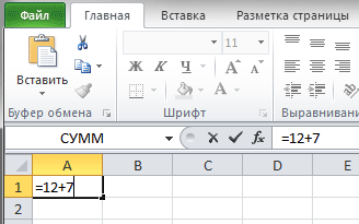
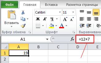
To find out what a cell actually contains - a formula or a number - you need to select it and look at the formula bar - the area located immediately above the column names. In our case, it just displays the formula that we just entered.
After carrying out all the operations, pay attention to the result of dividing the numbers 12 by 7, which is not an integer (1.714286) and contains quite a lot of digits after the decimal point. In most cases, such precision is not required, and such long numbers will only clutter the table.
To fix this, select the cell with the number for which you want to change the number of decimal places after the decimal point and on the tab home in Group Number select team Decrease bit depth. Each click on this button removes one character.
To the left of the team Decrease bit depth There is a button that performs the opposite operation - it increases the number of decimal places to display more accurate values.
Drawing up formulas
Now let's return to the budget table we created in the first part of this series.
.png)
At the moment, it records monthly personal expenses for specific items. For example, you can find out how much was spent on food in February or on car maintenance in March. But the total monthly expenses are not indicated here, although these indicators are the most important for many. Let's correct this situation by adding the line “Monthly expenses” at the bottom of the table and calculate its values.

To calculate the total expense for January in cell B7, you can write the following expression: “=18250+5100+6250+2500+3300” and press Enter, after which you will see the result of the calculation. This is an example of using a simple formula, the compilation of which is no different from calculations on a calculator. Unless the equal sign is placed at the beginning of the expression, and not at the end.
Now imagine that you made a mistake when indicating the values of one or more expense items. In this case, you will have to adjust not only the data in the cells indicating expenses, but also the formula for calculating total expenses. Of course, this is very inconvenient and therefore in Excel, when creating formulas, not specific numerical values are often used, but cell addresses and ranges.
With this in mind, let's change our formula for calculating total monthly expenses.

In cell B7, enter an equal sign (=) and... Instead of manually entering the value of cell B2, left-click on it. After this, a dotted highlight frame will appear around the cell, which indicates that its value is included in the formula. Now enter the “+” sign and click on cell B3. Next, do the same with cells B4, B5 and B6, and then press the ENTER key, after which the same amount value will appear as in the first case.
Select cell B7 again and look at the formula bar. It can be seen that instead of numbers - cell values, the formula contains their addresses. This is a very important point, since we just built a formula not from specific numbers, but from cell values that can change over time. For example, if you now change the amount of expenses for purchasing things in January, then the entire monthly total expense will be recalculated automatically. Give it a try.
Now let's assume that you need to sum not five values, as in our example, but one hundred or two hundred. As you understand, using the above method of constructing formulas in this case is very inconvenient. In this case, it is better to use the special “AutoSum” button, which allows you to calculate the sum of several cells within one column or row. In Excel, you can calculate not only the sums of columns, but also rows, so we use it to calculate, for example, total food expenses for six months.

Place the cursor on an empty cell on the side of the desired line (in our case it is H2). Then click the button Sum on the bookmark home in Group Editing. Now, let's go back to the table and see what happened.

In the cell we selected, a formula appears with a range of cells whose values need to be summed. At the same time, the dotted highlight frame appeared again. Only this time it frames not just one cell, but the entire range of cells, the sum of which needs to be calculated.
Now let's look at the formula itself. As before, the equals sign comes first, but this time it is followed by function“SUM” is a predefined formula that will add the values of the specified cells. Immediately after the function there are brackets located around the addresses of the cells whose values need to be summed, called formula argument. Please note that the formula does not indicate all the addresses of the cells being summed, but only the first and last ones. The colon between them indicates that range cells from B2 to G2.
After pressing Enter, the result will appear in the selected cell, but that’s all the button can do Sum don't end. Click on the arrow next to it and a list will open containing functions for calculating average values (Average), the number of data entered (Number), maximum (Maximum) and minimum (Minimum) values.

So, in our table we calculated the total expenses for January and the total expenses on food for six months. At the same time, they did this in two different ways - first using cell addresses in the formula, and then using functions and ranges. Now, it's time to finish the calculations for the remaining cells, calculating the total costs for the remaining months and expense items.
Autofill
To calculate the remaining amounts, we will use one remarkable feature of Excel, which is the ability to automate the process of filling cells with systematic data.
Sometimes in Excel you have to enter similar data of the same type in a certain sequence, for example, days of the week, dates, or row numbers. Remember, in the first part of this series, in the table header, we entered the name of the month in each column separately? In fact, it was completely unnecessary to enter this entire list manually, since the application can do it for you in many cases.
Let's erase all the month names in the header of our table, except for the first one. Now select the cell labeled “January” and move the mouse pointer to its lower right corner so that it takes the form of a cross called fill marker. Hold down the left mouse button and drag it to the right.
.png)
A tooltip will appear on the screen, telling you the value the program is about to insert into the next cell. In our case, this is “February”. As you move the marker down, it will change to the names of other months, which will help you figure out where to stop. Once the button is released, the list will populate automatically.
Of course, Excel does not always correctly “understand” how to fill in subsequent cells, since the sequences can be quite diverse. Let's imagine that we need to fill a line with even numeric values: 2, 4, 6, 8 and so on. If we enter the number “2” and try to move the autofill marker to the right, it turns out that the program offers to insert the value “2” again both in the next and in other cells.
 In this case, the application needs to provide a little more data. To do this, in the next cell on the right, enter the number “4”. Now select both filled cells and again move the cursor to the lower right corner of the selection area so that it takes the form of a selection marker. Moving the marker down, we see that the program has now understood our sequence and is showing the required values in the tooltips.
Thus, for complex sequences, before using autofill, you need to fill in several cells yourself so that Excel can correctly determine the general algorithm for calculating their values.
Now let's apply this useful program feature to our table, so that we can enter formulas manually for the remaining cells. First, select the cell with the amount already calculated (B7).

Now “hook” the cursor on the lower right corner of the square and drag the marker to the right to cell G7. After you release the key, the application itself will copy the formula into the marked cells, while automatically changing the addresses of the cells contained in the expression, substituting the correct values.
Moreover, if the marker is moved to the right, as in our case, or down, then the cells will be filled in ascending order, and to the left or up - in descending order.
There is also a way to fill a row using tape. Let's use it to calculate the cost amounts for all expense items (column H).

We select the range that should be filled, starting from the cell with the data already entered. Then on the tab home in Group Editing press the button Fill and select the filling direction.
Add rows, columns, and merge cells
To get more practice in writing formulas, let's expand our table and at the same time learn a few basic formatting operations. For example, let’s add income items to the expenditure side, and then calculate possible budget savings.
Let's assume that the revenue part of the table will be located on top of the expenditure part. To do this we will have to insert a few extra lines. As always, this can be done in two ways: using commands on the ribbon or in the context menu, which is faster and easier.
Right-click in any cell of the second row and select the command from the menu that opens Insert…, and then in the window - Add line.

After inserting a row, pay attention to the fact that by default it is inserted above the selected row and has the format (cell background color, size settings, text color, etc.) of the row located above it.

If you need to change the default formatting, immediately after pasting, click the button Add Options icon that automatically appears near the lower right corner of the selected cell and select the option you want.
Using a similar method, you can insert columns into the table that will be placed to the left of the selected one and individual cells.
By the way, if a row or column ends up in the wrong place after insertion, you can easily delete it. Right-click on any cell belonging to the object to be deleted and select the command from the menu that opens Delete. Finally, indicate what exactly you want to delete: a row, a column, or an individual cell.
On the ribbon, you can use the button for adding operations Insert located in the group Cells on the bookmark home, and to delete, the command of the same name in the same group.
In our case, we need to insert five new rows at the top of the table immediately after the header. To do this, you can repeat the adding operation several times, or you can, having completed it once, use the “F4” key, which repeats the most recent operation.
As a result, after inserting five horizontal rows into the top part of the table, we bring it to the following form:

We left the white unformatted rows in the table on purpose to separate the income, expenditure and total parts from each other by writing appropriate headings in them. But before we do that, we will learn one more operation in Excel - merging cells.
When several adjacent cells are combined, one is formed, which can occupy several columns or rows at once. In this case, the name of the merged cell becomes the address of the uppermost cell of the merged range. At any time, you can split a merged cell again, but you cannot split a cell that has never been merged.
When merging cells, only the data in the top left is saved, but the data in all other merged cells will be deleted. Remember this and do the merging first, and only then enter the information.
Let's return to our table. In order to write headings in white lines, we need only one cell, while now they consist of eight. Let's fix this. Select all eight cells of the second row of the table and on the tab home in Group Alignment click on the button Combine and place in the center.

After executing the command, all selected cells in the row will be combined into one large cell.
Next to the merge button there is an arrow, clicking on which will bring up a menu with additional commands that allow you to: merge cells without central alignment, merge entire groups of cells horizontally and vertically, and also cancel the merge.
After adding headers, as well as filling out the lines: salary, bonuses and monthly income, our table began to look like this:
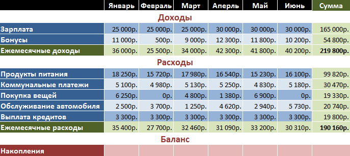
Conclusion
In conclusion, let's calculate the last line of our table, using the knowledge gained in this article, the cell values of which will be calculated using the following formula. In the first month, the balance will be the normal difference between the income received for the month and the total expenses in it. But in the second month we will add the balance of the first to this difference, since we are calculating savings. Calculations for subsequent months will be carried out according to the same scheme - savings for the previous period will be added to the current monthly balance.
Now let's translate these calculations into formulas that Excel can understand. For January (cell B14) the formula is very simple and will look like this: “=B5-B12”. But for cell C14 (February), the expression can be written in two different ways: “=(B5-B12)+(C5-C12)” or “=B14+C5-C12”. In the first case, we again calculate the balance of the previous month and then add the balance of the current month to it, and in the second, the already calculated result for the previous month is included in the formula. Of course, using the second option to construct the formula in our case is much preferable. After all, if you follow the logic of the first option, then in the expression for the March calculation there will already be 6 cell addresses, in April - 8, in May - 10, and so on, and when using the second option there will always be three of them.
To fill the remaining cells from D14 to G14, we will use the ability to fill them automatically, just as we did in the case of amounts.
By the way, to check the value of the final savings for June, located in cell G14, in cell H14 you can display the difference between the total amount of monthly income (H5) and monthly expenses (H12). As you understand, they should be equal.
As can be seen from the latest calculations, in formulas you can use not only the addresses of adjacent cells, but also any others, regardless of their location in the document or belonging to a particular table. Moreover, you have the right to link cells located on different sheets of the document and even in different books, but we will talk about this in the next publication.
And here is our final table with the calculations performed:

Now, if you wish, you can continue filling it out yourself, inserting both additional items of expenses or income (rows) and adding new months (columns).
In the next article we will talk in more detail about functions, understand the concept of relative and absolute links, be sure to master several more useful elements of table editing, and much more.
Anyone who uses a computer in their daily work has, in one way or another, encountered the Excel office application, which is part of the standard Microsoft Office package. It is available in any version of the package. And quite often, when starting to get acquainted with the program, many users wonder whether they can use Excel on their own?
What is Excel?
First, let's define what Excel is and what this application is needed for. Many people have probably heard that the program is a spreadsheet editor, but the principles of its operation are fundamentally different from the same tables created in Word.
If in Word a table is more of an element in which a text or table is displayed, then a sheet with an Excel table is, in fact, a unified mathematical machine that is capable of performing a wide variety of calculations based on specified data types and formulas by which this or that mathematical or algebraic operation.
How to learn to work in Excel on your own and is it possible to do it?
As the heroine of the film “Office Romance” said, you can teach a hare to smoke. In principle, nothing is impossible. Let's try to understand the basic principles of the application's functioning and focus on understanding its main capabilities.
Of course, reviews from people who understand the specifics of the application say that you can, say, download some tutorial on how to work in Excel, however, as practice shows, and especially the comments of novice users, such materials are very often presented in a too abstruse form, and It can be quite difficult to figure out.
It seems that the best training option would be to study the basic capabilities of the program, and then apply them, so to speak, “by scientific poking.” It goes without saying that you first need to consider the basic functional elements of Microsoft Excel (the program lessons indicate exactly this) in order to get a complete picture of the principles of operation.
Key elements to pay attention to
The very first thing the user pays attention to when launching the application is a sheet in the form of a table, in which cells are located, numbered in different ways, depending on the version of the application itself. In earlier versions, columns were designated by letters, and rows by numbers and numbers. In other releases, all markings are presented exclusively in digital form.

What is it for? Yes, only so that it is always possible to determine the cell number for specifying a certain calculation operation, similar to how coordinates are specified in a two-dimensional system for a point. Later it will be clear how to work with them.
Another important component is the formula bar - a special field with an “f x” icon on the left. This is where all operations are specified. At the same time, the mathematical operations themselves are designated in exactly the same way as is customary in the international classification (equal sign “=”, multiplication “*” division “/”, etc.). Trigonometric quantities also correspond to international notations (sin, cos, tg, etc.). But this is the simplest thing. More complex operations will have to be mastered with the help of the help system or specific examples, since some formulas may look quite specific (exponential, logarithmic, tensor, matrix, etc.).
At the top, as in other office programs, there is the main panel and the main menu sections with the main operation items and quick access buttons to a particular function.
and simple operations with them
Consideration of the question is impossible without a key understanding of the types of data entered in table cells. Let us immediately note that after entering some information, you can press the enter button, the Esc key, or simply move the rectangle from the desired cell to another - the data will be saved. Editing a cell is done by double-clicking or pressing the F2 key, and upon completion of data entry, saving occurs only by pressing the Enter key.

Now a few words about what can be entered in each cell. The format menu is called up by right-clicking on the active cell. On the left there is a special column indicating the data type (general, numeric, text, percentage, date, etc.). If the general format is selected, the program, roughly speaking, itself determines what exactly the entered value looks like (for example, if you enter 01/01/16, the date January 1, 2016 will be recognized).

When entering a number, you can also use an indication of the number of decimal places (by default, one character is displayed, although when entering two, the program simply rounds the visible value, although the true value does not change).
When using, say, a text data type, whatever the user types will be displayed exactly as typed on the keyboard, without modification.
Here's what's interesting: if you hover the cursor over the selected cell, a cross will appear in the lower right corner, by pulling it while holding down the left mouse button, you can copy the data to the cells following the desired one in order. But the data will change. If we take the same date example, the next value would be January 2, and so on. This type of copying can be useful when specifying the same formula for different cells (sometimes even with cross calculations).
When it comes to formulas, for the simplest operations you can use a two-pronged approach. For example, for the sum of cells A1 and B1, which must be calculated in cell C1, you need to place the rectangle in the C1 field and specify the calculation using the formula “=A1+B1”. You can do it differently by setting the equality “=SUM(A1:B1)” (this method is more used for large gaps between cells, although you can use the automatic sum function, as well as the English version of the SUM command).
Excel program: how to work with Excel sheets
When working with sheets, you can perform many actions: add sheets, change their names, delete unnecessary ones, etc. But the most important thing is that any cells located on different sheets can be interconnected by certain formulas (especially when large amounts of information of different types are entered).

How to learn to work in Excel on your own in terms of use and calculations? It's not that simple here. As reviews from users who have mastered this spreadsheet editor show, it will be quite difficult to do this without outside help. You should at least read the help system of the program itself. The simplest way is to enter cells in the same formula by selecting them (this can be done both on one sheet and on different ones. Again, if you enter the sum of several fields, you can enter “=SUM”, and then simply select one by one while holding down the Ctrl key the necessary cells.But this is the most primitive example.
Additional features
But in the program you can not only create tables with various types of data. Based on them, in a couple of seconds you can build all kinds of graphs and diagrams by specifying either a selected range of cells for automatic construction, or specifying it manually when entering the corresponding menu.

In addition, the program has the ability to use special add-ons and executable scripts based on Visual Basic. You can insert any objects in the form of graphics, video, audio or anything else. In general, there are enough opportunities. And here only a small fraction of everything that this unique program is capable of is touched upon.
What can I say, with the right approach, it can calculate matrices, solve all kinds of equations of any complexity, find, create databases and connect them with other applications like Microsoft Access and much more - you just can’t list it all.
Bottom line
Now, it’s probably already clear that the question of how to learn to work in Excel on your own is not so easy to consider. Of course, if you master the basic principles of working in the editor, setting the simplest operations will not be difficult. User reviews indicate that you can learn this in a maximum of a week. But if you need to use more complex calculations, and even more so, work with reference to databases, no matter how much anyone wants it, you simply cannot do without special literature or courses. Moreover, it is very likely that you will even have to improve your knowledge of algebra and geometry from the school course. Without this, you can’t even dream of fully using the spreadsheet editor.